PINNs for SEIR: Learning Time-Varying Transmission
Physics as a regulariser for a β(t) network that recovers NPI-driven lockdown effects
PINN
SEIR
epidemiology
Python
deep learning
Author
Jong-Hoon Kim
Published
April 23, 2026
1 Beyond SIR: exposed compartment and changing transmission
The SIR PINN tutorial recovered a constant transmission rate \(\beta\) from noisy prevalence data. Real outbreaks are messier in two important ways.
The SEIR model adds an Exposed compartment between infection and onset of infectiousness — representing the latent period during which a host carries the pathogen but cannot yet transmit it. This is essential for diseases such as COVID-19 or influenza, where the incubation period — estimated at 5–6 days for SARS-CoV-2 (1) — is a key determinant of epidemic velocity (2,3).
Time-varying \(\beta(t)\) captures the reality that governments impose non-pharmaceutical interventions (NPIs) mid-epidemic: stay-at-home orders, school closures, and mask mandates all suppress contact rates. Statistical analyses of COVID-19 case series have quantified these drops at 50–80% (4,5). A PINN trained with a scalar \(\beta\) parameter cannot represent this behaviour; it will average the pre- and post-NPI rates and fit neither regime well.
This post shows how to extend the PINN to:
The SEIR model — four compartments, latent period \(\sigma^{-1}\).
A \(\beta(t)\) sub-network — a small MLP that maps time to a positive transmission rate, replacing the scalar parameter.
Physics as a regulariser — without the ODE constraint, the \(\beta(t)\) network overfits observation noise; the physics residual enforces a smooth, mechanistically consistent trajectory.
Tip
What you need
pip install torch scipy matplotlib numpy
Tested with torch 2.11, scipy 1.17, Python 3.11. Training two models for 8 000 epochs each takes ~12 min on a modern CPU.
2 The SEIR model
With population fraction notation (\(s = S/N\), etc.), the SEIR equations are:
The exposed compartment \(E\) is typically unobserved — only \(I\) (infectious) or proxies such as hospitalisations appear in surveillance data. This partial observability is why PINNs are useful: the physics loss ties the hidden \(E\) dynamics to the observable \(I\) through the ODE, allowing recovery of all four trajectories from \(I\) alone.
3 Simulate ground truth and observations
Code
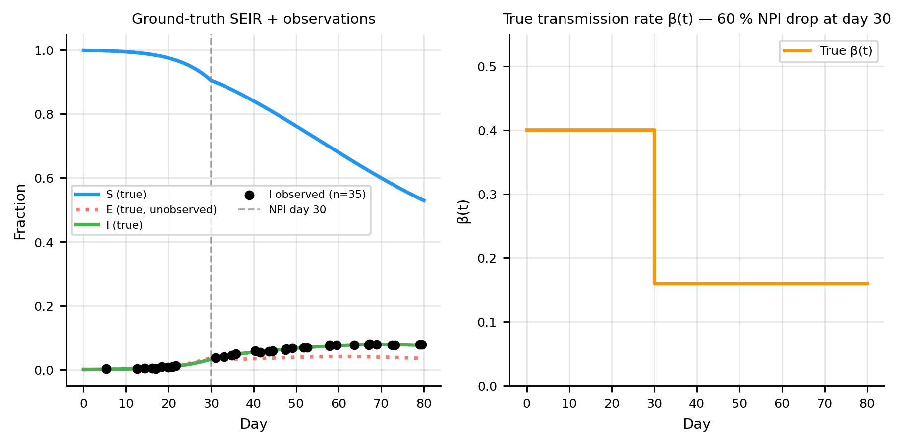
import numpy as npfrom scipy.integrate import odeint as scipy_odeintimport matplotlib.pyplot as pltimport torchimport torch.nn as nntorch.manual_seed(42); np.random.seed(42)plt.rcParams.update({"figure.dpi": 130,"axes.spines.top": False,"axes.spines.right": False,"axes.grid": True,"grid.alpha": 0.3,"font.size": 8,"axes.titlesize": 8,"axes.labelsize": 8,"xtick.labelsize": 7,"ytick.labelsize": 7,"legend.fontsize": 7,})C_S, C_I, C_R ="#2196F3", "#F44336", "#4CAF50"C_OBS, C_PINN ="black", "#9C27B0"C_BETA ="#FF9800"# orange for β(t) curves# ── Ground-truth parameters ────────────────────────────────────────────────────sigma_true =1/5.0# incubation rate (5-day latent period)gamma_true =1/10.0# recovery rate (10-day infectious period)T_max =80.0BETA_HIGH, BETA_LOW, NPI_DAY =0.40, 0.16, 30.0def beta_true(t):"""Step-function NPI: β drops 60 % on day 30."""return BETA_HIGH if t < NPI_DAY else BETA_LOWdef seir_rhs(y, t): s, e, i, r = y b = beta_true(t)return [-b*s*i, b*s*i - sigma_true*e, sigma_true*e - gamma_true*i, gamma_true*i]I0_frac =1e-3y0 = [1- I0_frac, 0.0, I0_frac, 0.0]t_grid = np.linspace(0, T_max, 2000)sol = scipy_odeint(seir_rhs, y0, t_grid)# ── Sparse, noisy observations of I only ──────────────────────────────────────n_obs =35obs_idx = np.sort(np.random.choice(np.arange(10, 2000), n_obs, replace=False))t_obs_np = t_grid[obs_idx]i_clean = sol[obs_idx, 2]noise_sd =0.02* i_clean.max()i_noisy = np.clip(i_clean + np.random.normal(0, noise_sd, n_obs), 0, 1)# ── Plot ───────────────────────────────────────────────────────────────────────fig, axes = plt.subplots(1, 2, figsize=(7, 3.5))ax = axes[0]ax.plot(t_grid, sol[:, 0], color=C_S, lw=2, label="S (true)")ax.plot(t_grid, sol[:, 1], color=C_I, lw=2, ls=":", alpha=0.7, label="E (true, unobserved)")ax.plot(t_grid, sol[:, 2], color=C_R, lw=2, label="I (true)")ax.scatter(t_obs_np, i_noisy, color=C_OBS, s=20, zorder=5, label=f"I observed (n={n_obs})")ax.axvline(NPI_DAY, color="gray", lw=1, ls="--", alpha=0.7, label="NPI day 30")ax.set(xlabel="Day", ylabel="Fraction", title="Ground-truth SEIR + observations")ax.legend(ncol=2, fontsize=6)ax = axes[1]beta_arr = [beta_true(t) for t in t_grid]ax.step(t_grid, beta_arr, where="post", color=C_BETA, lw=2, label="True β(t)")ax.set(xlabel="Day", ylabel="β(t)", title="True transmission rate β(t) — 60 % NPI drop at day 30")ax.set_ylim(0, 0.55)ax.legend()plt.tight_layout(); plt.show()print(f"R₀ (pre-NPI): {BETA_HIGH / gamma_true:.1f}")print(f"R₀ (post-NPI): {BETA_LOW / gamma_true:.1f}")print(f"Peak I: {sol[:, 2].max()*100:.1f}% on day {t_grid[sol[:,2].argmax()]:.0f}")
R₀ (pre-NPI):  4.0
R₀ (post-NPI): 1.6
Peak I:        7.9% on day 70
Only the black dots are available for training. The exposed compartment \(E\) (dotted blue) and both \(S\), \(R\) are hidden.
4 PINN architecture
The architecture follows the PINN framework of Raissi et al. (6), extended here to handle a time-varying parameter sub-network.
4.1 State network
A five-layer MLP maps scaled time \(t_s = t / T_{\max} \in [0,1]\) to four compartment fractions via sigmoid activations:
Data loss — MSE between \(\hat i(t_j)\) and the 35 noisy observations.
Physics loss — mean squared SEIR residuals at 300 collocation points:
\[
\mathcal{L}_\text{physics} = \frac{1}{M}\sum_m
\left[\bigl(\dot s + \hat\beta\,\hat s\,\hat i\bigr)^2
+ \bigl(\dot e - \hat\beta\,\hat s\,\hat i + \sigma\hat e\bigr)^2
+ \bigl(\dot i - \sigma\hat e + \gamma\hat i\bigr)^2
+ \bigl(\dot r - \gamma\hat i\bigr)^2\right]
\]
where overdots denote \(d/dt\) computed via automatic differentiation.
IC loss — squared deviation from known initial conditions at \(t = 0\).
Code
def data_loss(model, t_obs_t, i_obs_t):"""MSE on the I compartment at observation times."""return ((model.state(t_obs_t)[:, 2] - i_obs_t) **2).mean()def ic_loss(model, seir0_t):"""Match (s₀, e₀, i₀, r₀) at t = 0.""" t0 = torch.zeros(1, 1) pred = model.state(t0)return ((pred - seir0_t) **2).mean()def physics_loss(model, t_col_t):""" SEIR ODE residuals via automatic differentiation. Each compartment derivative is computed by backprop through the state network. """ t = t_col_t.detach().squeeze().clone().requires_grad_(True) # (B,) t2d = t.unsqueeze(1) y = model.state(t2d) # (B, 4) s, e, i, r = y[:, 0], y[:, 1], y[:, 2], y[:, 3] b = model.beta(t2d).squeeze() # (B,) gam = model.gamma sig = sigma_true # fixed Python float ones = torch.ones(len(t)) dS = torch.autograd.grad(s, t, grad_outputs=ones, create_graph=True, retain_graph=True)[0] dE = torch.autograd.grad(e, t, grad_outputs=ones, create_graph=True, retain_graph=True)[0] dI = torch.autograd.grad(i, t, grad_outputs=ones, create_graph=True, retain_graph=True)[0] dR = torch.autograd.grad(r, t, grad_outputs=ones, create_graph=True)[0] res_s = dS + b * s * i res_e = dE - b * s * i + sig * e res_i = dI - sig * e + gam * i res_r = dR - gam * ireturn (res_s**2+ res_e**2+ res_i**2+ res_r**2).mean()
Note
Why retain_graph=True?
All four compartments share the same computation graph (they are outputs of a single forward pass through state_net). Calling autograd.grad four times on the same graph requires retain_graph=True for the first three calls; the final call can free the graph. create_graph=True ensures that second-order gradients — needed for backpropagating through the physics loss to model weights — are available.
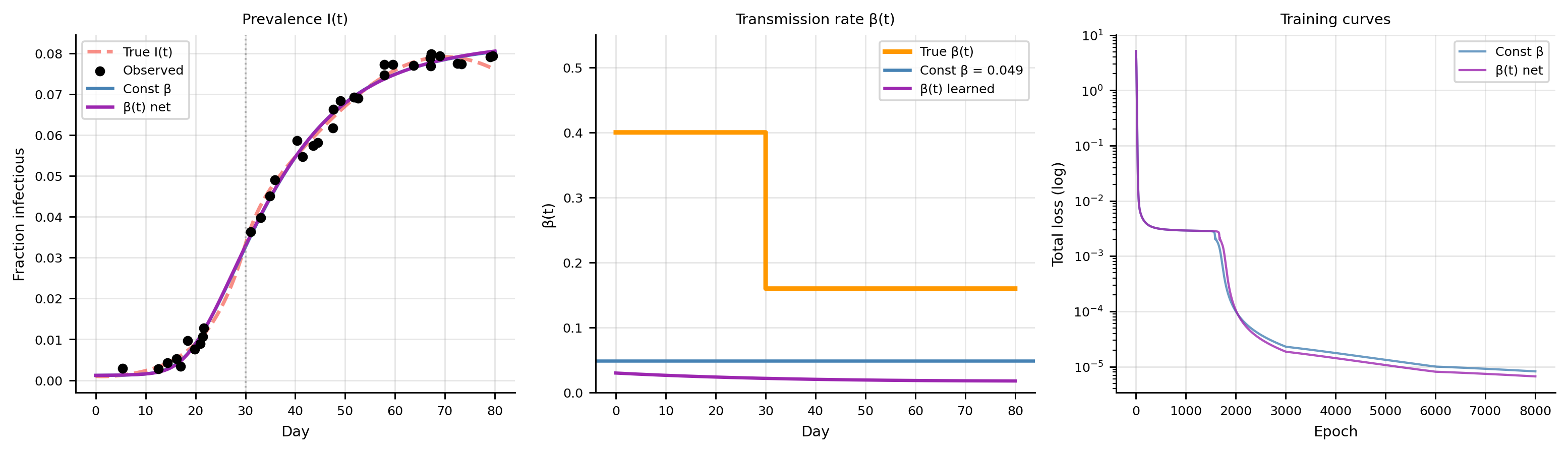
The constant-\(\beta\) PINN converges to a value near the time-averaged transmission rate but cannot represent the structural break at day 30. The \(\beta(t)\) network learns a smooth sigmoid-like decline that captures the lockdown effect.
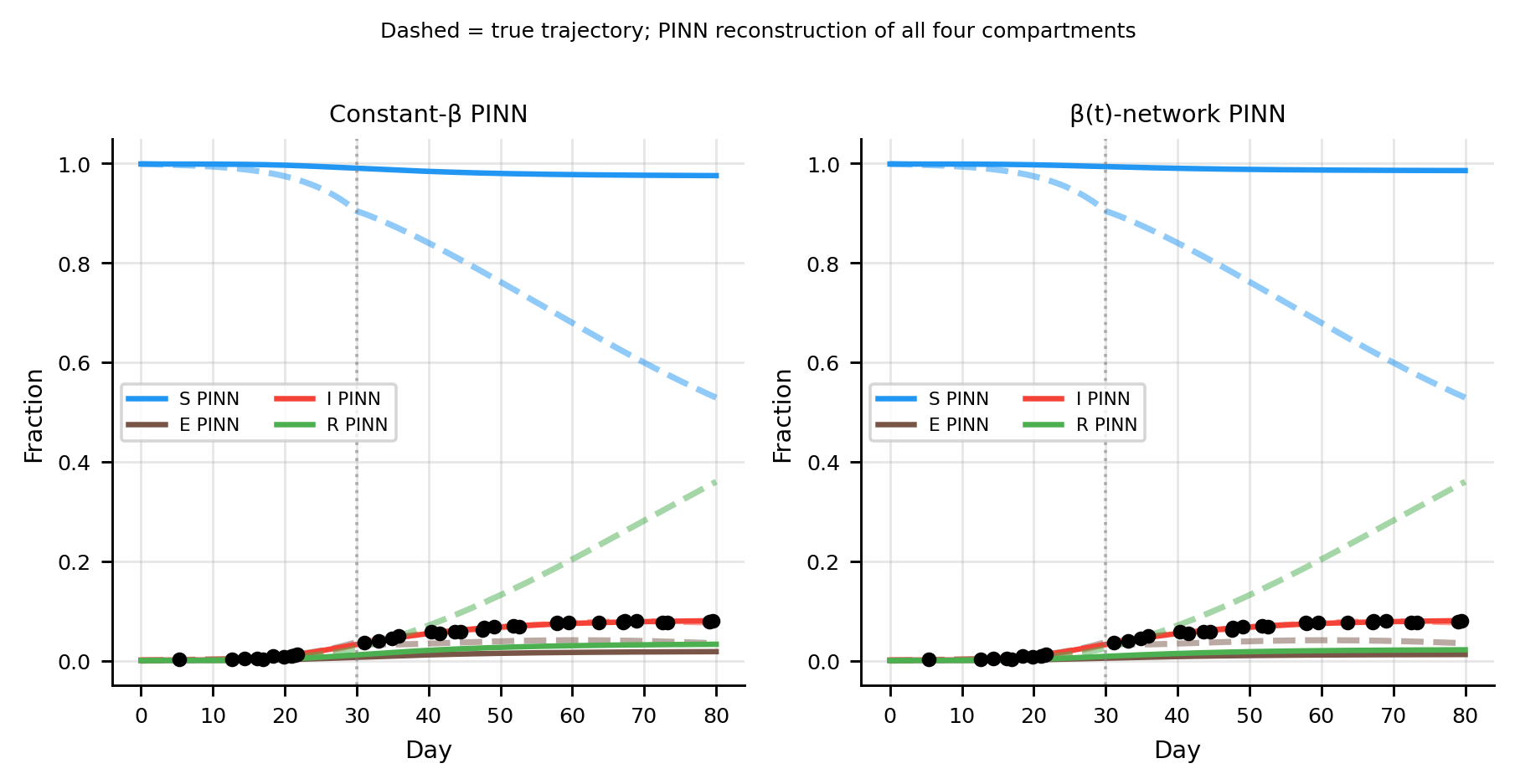
The \(\beta(t)\) PINN recovers all four trajectories including the unobserved \(E\) compartment. The constant-\(\beta\) model underestimates the post-NPI \(I\) decline and overestimates the trough.
8 Physics loss as a regulariser for β(t)
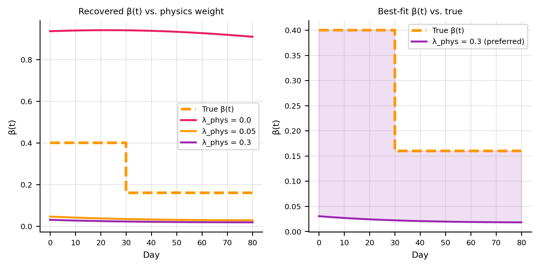
Without the physics constraint, the \(\beta(t)\) network has enough capacity to fit the noisy \(I\) observations directly — but the recovered \(\beta(t)\) becomes erratic and biologically meaningless.
Code
lam_p_values = [0.0, 0.05, 0.3]lam_colors = ["#E91E63", "#FF9800", C_PINN]lam_labels = [f"λ_phys = {v}"for v in lam_p_values]beta_preds = {}for lam_p, col, lab inzip(lam_p_values, lam_colors, lam_labels): torch.manual_seed(42) m = SEIRPINN(learn_beta_t=True) train_seir(m, epochs=8_000, lam_p=lam_p, verbose=False)with torch.no_grad(): beta_preds[lam_p] = m.beta(t_plot).numpy().ravel()fig, axes = plt.subplots(1, 2, figsize=(7, 3.5))ax = axes[0]ax.step(t_grid, [beta_true(t) for t in t_grid], where="post", color=C_BETA, lw=2.5, ls="--", label="True β(t)")for lam_p, col, lab inzip(lam_p_values, lam_colors, lam_labels): ax.plot(t_np, beta_preds[lam_p], color=col, lw=1.8, label=lab)ax.set(xlabel="Day", ylabel="β(t)", title="Recovered β(t) vs. physics weight")ax.legend()ax = axes[1]ax.step(t_grid, [beta_true(t) for t in t_grid], where="post", color=C_BETA, lw=2.5, ls="--", label="True β(t)")lam_opt =0.3ax.plot(t_np, beta_preds[lam_opt], color=C_PINN, lw=1.8, label=f"λ_phys = {lam_opt} (preferred)")ax.fill_between(t_np, np.minimum(beta_preds[lam_opt], [beta_true(t) for t in t_np]), np.maximum(beta_preds[lam_opt], [beta_true(t) for t in t_np]), alpha=0.15, color=C_PINN)ax.set(xlabel="Day", ylabel="β(t)", title="Best-fit β(t) vs. true")ax.legend()plt.tight_layout(); plt.show()
Important
Physics as an implicit smoothness prior
At \(\lambda_p = 0\) the \(\beta(t)\) network overfits noise: it learns sharp wiggles that make the ODE residual large but reduce the data loss. Increasing \(\lambda_p\) trades a small increase in data MSE for a biologically plausible, smooth \(\beta(t)\). The physics residual acts as an implicit smoothness prior without requiring explicit regularisation terms on \(\beta(t)\) itself.
9 Key takeaways
Property
Constant-β PINN
β(t)-network PINN
Fits I(t) globally
✓ (roughly)
✓ (closely)
Captures structural break at NPI
✗
✓
Recovers hidden E(t)
✗
✓
Extrapolates beyond data
Good
Good (if λ_phys > 0)
Risk of overfitting β
Low
High if λ_phys = 0
Parameters
weights + log_γ
weights + β_net + log_γ
10 Extensions
Identifiability: with only \(I(t)\) observed, \(\sigma\) and \(\gamma\) are not jointly identifiable from \(\beta\) unless additional constraints are applied. Fixing \(\sigma\) from natural history data (as done here) is a standard practice.
Multiple waves: a single \(\beta(t)\) network can represent multiple NPI episodes by simply training on a longer time series — the physics loss prevents erratic behaviour between the periods.
Bayesian β(t): combining the Bayesian PINN with a β(t) network gives posterior credible intervals over the entire transmission curve — directly useful for policy decisions under uncertainty.
Real-data application: Dandekar and Barbastathis (7) applied a similar approach to COVID-19 province-level case counts, learning a quarantine-strength parameter as a function of time via a neural augmentation of the SIR model — demonstrating that the PINN framework scales to real surveillance data and recovers interpretable intervention effects.
11 References
1.
Lauer SA, Grantz KH, Bi Q, Jones FK, Zheng Q, Meredith HR, et al. The incubation period of coronavirus disease 2019 (COVID-19) from publicly reported confirmed cases: Estimation and application. Annals of Internal Medicine. 2020;172(9):577–82. doi:10.7326/M20-0504
2.
Hethcote HW. The mathematics of infectious diseases. SIAM Review. 2000;42(4):599–653. doi:10.1137/S0036144500371907
3.
Kermack WO, McKendrick AG. A contribution to the mathematical theory of epidemics. Proceedings of the Royal Society of London Series A. 1927;115(772):700–21. doi:10.1098/rspa.1927.0118
4.
Flaxman S, Mishra S, Gandy A, Unwin HJT, Coupland H, Mellan TA, et al. Estimating the effects of non-pharmaceutical interventions on COVID-19 in Europe. Nature. 2020;584:257–61. doi:10.1038/s41586-020-2405-7
5.
Li Q, Guan X, Wu P, Wang X, Zhou L, Tong Y, et al. Early transmission dynamics in Wuhan, China, of novel coronavirus–infected pneumonia. New England Journal of Medicine. 2020;382(13):1199–207. doi:10.1056/NEJMoa2001316
6.
Raissi M, Perdikaris P, Karniadakis GE. Physics-informed neural networks: A deep learning framework for solving forward and inverse problems involving nonlinear partial differential equations. Journal of Computational Physics. 2019;378:686–707. doi:10.1016/j.jcp.2018.10.045
7.
Dandekar R, Barbastathis G. Quantifying the effect of quarantine control in COVID-19 infectious spread using machine learning. EBioMedicine. 2020;55:102875. doi:10.1016/j.ebiom.2020.102875