---
title: "Understanding Automatic Differentiation"
subtitle: "The derivative engine behind neural networks, backpropagation, and PINNs"
author: "Jong-Hoon Kim"
date: "2026-04-20"
categories: [automatic differentiation, deep learning, PINN, backpropagation, Python]
jupyter: python3
bibliography: references.bib
csl: https://www.zotero.org/styles/vancouver
format:
html:
toc: true
number-sections: true
code-fold: show
code-tools: true
execute:
echo: true
warning: false
message: false
---
In my [previous post on Physics-Informed Neural Networks](https://www.jonghoonk.com/blog/posts/pinn_sir/), the SIR residual was computed with a single line:
```python
dS = torch.autograd.grad(S, t, grad_outputs=ones, create_graph=True)[0]
```
That line uses **automatic differentiation** (AD). It computes $dS/dt$ to machine precision for arbitrary networks in roughly the same time it takes to evaluate the network itself.
This post takes AD apart. We will implement two small but working autodiff engines — one in forward mode, one in reverse mode — and understand exactly what PyTorch is doing when we call `.backward()` or `torch.autograd.grad(...)`.
---
# Why automatic differentiation matters
Modern deep learning is gradient descent on composed functions. Two places where derivatives show up in a typical PINN pipeline:
**Parameter gradients for training.** If $\mathcal{L}(\theta)$ is the loss and $\theta$ contains millions of network weights, we need $\nabla_\theta \mathcal{L}$ to update the weights with Adam or SGD.
**Derivatives inside the loss itself.** For a PINN solving the SIR ODE, the physics loss involves $dS/dt, dI/dt, dR/dt$ — derivatives of the *network output* with respect to the *network input*. These are computed through the same AD machinery.
Both cases reduce to one question: given a program that computes a numerical function, can we obtain its derivatives automatically, exactly, and efficiently? The answer is yes, and the mechanism is AD.
---
# Three ways to differentiate
Suppose we have the following function:
$$
f(x_1, x_2) = \ln(x_1) + x_1 x_2 - \sin(x_2).
$$
There are three ways a computer might compute $\partial f / \partial x_1$ at, say, $x_1 = 2, x_2 = 5$.
## Symbolic differentiation
Apply differentiation rules to the expression itself:
$$
\frac{\partial f}{\partial x_1} = \frac{1}{x_1} + x_2.
$$
This is what Mathematica and SymPy do. It returns a formula that we then evaluate. The problem is that repeated application of the product and chain rules on deep compositions produces expressions that grow exponentially. Symbolic differentiation of a neural network with a million parameters is not feasible.
## Numerical differentiation
Use a finite-difference approximation:
$$
\frac{\partial f}{\partial x_1}(x_1, x_2) \approx \frac{f(x_1 + h, x_2) - f(x_1, x_2)}{h}
$$
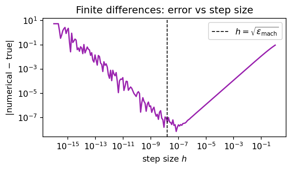
for small $h$. This is easy to implement but suffers from a fundamental tension between two errors:
- **Truncation error** $\sim O(h)$ (or $O(h^2)$ for centred differences): shrinks as $h \to 0$.
- **Round-off error** $\sim O(\epsilon_{\text{mach}}/h)$: grows as $h \to 0$, because we subtract two nearly equal numbers in floating point.
Minimising the sum gives an optimal $h \approx \sqrt{\epsilon_{\text{mach}}} \approx 10^{-8}$ in double precision:
```{python}
#| code-fold: true
#| fig-cap: "Total error of a forward finite difference versus step size, showing the classic U-curve."
import numpy as np
import matplotlib.pyplot as plt

def f(x):        return np.log(x) + x * 5 - np.sin(5.0)
def f_prime(x):  return 1.0 / x + 5                # analytic

x0 = 2.0
hs = np.logspace(-16, 0, 200)
fd = (f(x0 + hs) - f(x0)) / hs
err = np.abs(fd - f_prime(x0))

fig, ax = plt.subplots(figsize=(5, 3))
ax.loglog(hs, err, lw=1.6, color="#9C27B0")
ax.axvline(np.sqrt(np.finfo(float).eps), color="black", ls="--", lw=1,
           label=r"$h = \sqrt{\epsilon_{\mathrm{mach}}}$")
ax.set(xlabel="step size $h$", ylabel="|numerical − true|",
       title="Finite differences: error vs step size")
ax.legend()
plt.tight_layout()
plt.show()
```
Worse, computing the gradient of a function with $n$ inputs by finite differences requires $n+1$ function evaluations. For a network with a million parameters, that is a million forward passes per gradient step. Completely impractical.
## Automatic differentiation
AD sits between these two extremes. Like symbolic differentiation, it uses the chain rule exactly, so there is no truncation error. Unlike symbolic differentiation, it does not build a closed-form expression — it propagates *numerical derivative values* alongside the primal computation. The result: exact derivatives (to machine precision), at a cost comparable to a single function evaluation.
The trick is that every program — no matter how complex — is ultimately a composition of a small number of elementary operations ($+, \times, \sin, \exp, \log, \ldots$) whose derivatives we know by hand. AD applies the chain rule across this composition, one operation at a time.
---
# The computational graph
The program for $f(x_1, x_2) = \ln(x_1) + x_1 x_2 - \sin(x_2)$ can be written as a sequence of elementary operations:
$$
\begin{aligned}
v_1 &= x_1 \\
v_2 &= x_2 \\
v_3 &= \ln(v_1) \\
v_4 &= v_1 \cdot v_2 \\
v_5 &= \sin(v_2) \\
v_6 &= v_3 + v_4 \\
v_7 &= v_6 - v_5 \\
f &= v_7
\end{aligned}
$$
This is called a **Wengert list** or **trace**. We can draw it as a directed acyclic graph where edges indicate data flow:
```{mermaid}
flowchart LR
    x1((x₁)) --> v3["v₃ = ln(v₁)"]
    x1 --> v4["v₄ = v₁·v₂"]
    x2((x₂)) --> v4
    x2 --> v5["v₅ = sin(v₂)"]
    v3 --> v6["v₆ = v₃ + v₄"]
    v4 --> v6
    v6 --> v7["v₇ = v₆ - v₅"]
    v5 --> v7
    v7 --> f((f))
```
Every node corresponds to an elementary operation whose local derivative we know analytically. The chain rule tells us how to combine these local derivatives into the global derivative $\partial f / \partial x_i$. **This is the whole story.** What differs between *forward* and *reverse* mode AD is the order in which we traverse this graph.
---
# Forward mode: dual numbers
## Intuition
In forward mode, we propagate derivatives **alongside** values, in the same order as the original computation. At each node we carry a pair: the value $v_i$ (called the *primal*) and the derivative $\dot v_i = \partial v_i / \partial x_1$ with respect to some chosen input (called the *tangent*).
Initialise at the leaves:
- $v_1 = x_1, \quad \dot v_1 = 1$ (we are differentiating w.r.t. $x_1$)
- $v_2 = x_2, \quad \dot v_2 = 0$
Propagate forward using the chain rule at each node. For $v_4 = v_1 \cdot v_2$:
$$
\dot v_4 = \dot v_1 \cdot v_2 + v_1 \cdot \dot v_2.
$$
By the time we reach the output, $\dot f = \partial f / \partial x_1$ drops out.
| $i$ | $v_i$ | $\dot v_i$ (w.r.t. $x_1$) |
|-----|------------------|-------------------------------------|
| 1 | $x_1 = 2$ | $1$ |
| 2 | $x_2 = 5$ | $0$ |
| 3 | $\ln 2 = 0.693$ | $\dot v_1 / v_1 = 0.5$ |
| 4 | $2 \cdot 5 = 10$ | $\dot v_1 v_2 + v_1 \dot v_2 = 5$ |
| 5 | $\sin 5 = -0.959$| $\cos(v_2)\,\dot v_2 = 0$ |
| 6 | $10.693$ | $\dot v_3 + \dot v_4 = 5.5$ |
| 7 | $11.652$ | $\dot v_6 - \dot v_5 = 5.5$ |
So $\partial f / \partial x_1 = 5.5$, which matches the analytic answer $1/x_1 + x_2 = 0.5 + 5 = 5.5$.
## Dual numbers: an elegant implementation
Forward-mode AD has a stunning algebraic reformulation. Introduce a symbol $\varepsilon$ with the rule $\varepsilon^2 = 0$ (but $\varepsilon \neq 0$). A **dual number** is an expression $a + b\varepsilon$ where $a$ and $b$ are real. The arithmetic rules are:
$$
(a + b\varepsilon) + (c + d\varepsilon) = (a+c) + (b+d)\varepsilon
$$
$$
(a + b\varepsilon)(c + d\varepsilon) = ac + (ad + bc)\varepsilon + bd\,\varepsilon^2 = ac + (ad+bc)\varepsilon
$$
The magic: for any smooth $f$, the Taylor expansion gives
$$
f(a + b\varepsilon) = f(a) + f'(a) \cdot b\varepsilon + \tfrac{1}{2}f''(a) \cdot b^2 \varepsilon^2 + \cdots = f(a) + f'(a) b \varepsilon,
$$
because every term with $\varepsilon^2$ or higher vanishes. So if we evaluate $f$ on the dual number $x + \varepsilon$, the primal part is $f(x)$ and the dual part is $f'(x)$. **The derivative is computed as a by-product of a single function evaluation**, simply by running the ordinary code on dual numbers instead of floats.
## A working implementation in ~40 lines
```{python}
import math

class Dual:
    """Forward-mode AD via dual numbers: a + b·ε, ε² = 0."""

    def __init__(self, primal, tangent=0.0):
        self.primal  = primal
        self.tangent = tangent

    # ------------------------------------------------------------------
    # Elementary operator overloads
    # ------------------------------------------------------------------
    def __add__(self, other):
        o = other if isinstance(other, Dual) else Dual(other)
        return Dual(self.primal + o.primal, self.tangent + o.tangent)

    def __sub__(self, other):
        o = other if isinstance(other, Dual) else Dual(other)
        return Dual(self.primal - o.primal, self.tangent - o.tangent)

    def __mul__(self, other):
        o = other if isinstance(other, Dual) else Dual(other)
        return Dual(self.primal * o.primal,
                    self.primal * o.tangent + self.tangent * o.primal)

    def __truediv__(self, other):
        o = other if isinstance(other, Dual) else Dual(other)
        p = self.primal / o.primal
        t = (self.tangent * o.primal - self.primal * o.tangent) / o.primal**2
        return Dual(p, t)

    __radd__, __rsub__, __rmul__ = __add__, __sub__, __mul__

    def __repr__(self):
        return f"Dual({self.primal:.4f}, ε·{self.tangent:.4f})"

def sin(x):  return Dual(math.sin(x.primal),  math.cos(x.primal) * x.tangent)
def cos(x):  return Dual(math.cos(x.primal), -math.sin(x.primal) * x.tangent)
def exp(x):  return Dual(math.exp(x.primal),  math.exp(x.primal) * x.tangent)
def log(x):  return Dual(math.log(x.primal),  x.tangent / x.primal)

# ------------------------------------------------------------------
# Differentiate f(x1, x2) = ln(x1) + x1*x2 - sin(x2) at (2, 5)
# ------------------------------------------------------------------
def f(x1, x2):
    return log(x1) + x1 * x2 - sin(x2)

# Seed tangent on x1 to get ∂f/∂x1
x1 = Dual(2.0, 1.0)
x2 = Dual(5.0, 0.0)
print(f(x1, x2))   # primal = f(2,5), tangent = ∂f/∂x1

# Seed tangent on x2 to get ∂f/∂x2
x1 = Dual(2.0, 0.0)
x2 = Dual(5.0, 1.0)
print(f(x1, x2))
```
That is a complete, working autodiff system in about 40 lines. The mathematical content is identical to what PyTorch does in forward mode. The only thing missing is generalisation from scalars to tensors.
## When forward mode is efficient
Each forward pass seeds exactly one input. To get the full gradient of $f: \mathbb{R}^n \to \mathbb{R}$, we must run the computation $n$ times, once per input. Cost: $O(n) \times$ cost of evaluating $f$.
For a neural network with $n = 10^6$ parameters and a scalar loss, that is a million forward passes per gradient step — exactly the same problem finite differences had.
Forward mode is efficient in a different regime: **few inputs, many outputs**. Computing a Jacobian $J \in \mathbb{R}^{m \times n}$ column by column costs $O(n)$, but row by row costs $O(m)$. For deep learning, we want rows.
---
# Reverse mode: backpropagation
## Intuition
Reverse mode inverts the traversal. Instead of propagating $\partial v_i / \partial x_j$ forward from each input, we propagate $\partial f / \partial v_i$ **backward** from the output. This quantity is called the **adjoint** or **cotangent** of $v_i$ and is often written $\bar v_i$.
The chain rule, read backward: if $v_j$ depends on $v_i$ through the operation $v_j = \phi(v_i, \ldots)$, then $v_i$ contributes to $\bar v_j$ through $\partial v_j / \partial v_i$:
$$
\bar v_i \;=\; \sum_{j \,:\, v_j \text{ uses } v_i} \bar v_j \cdot \frac{\partial v_j}{\partial v_i}.
$$
Starting from $\bar f = 1$ and walking the graph backward, we accumulate $\bar v_i$ at each node. When we reach a leaf $x_k$, its adjoint is $\bar x_k = \partial f / \partial x_k$ — exactly the gradient we wanted.
The algorithm is two passes:
1. **Forward pass**: evaluate the program, recording each operation and its inputs onto a *tape*.
2. **Backward pass**: walk the tape in reverse, accumulating adjoints.
## Worked example on $f(x_1, x_2) = \ln(x_1) + x_1 x_2 - \sin(x_2)$
Forward pass at $(x_1, x_2) = (2, 5)$ produces $v_3 = 0.693, v_4 = 10, v_5 = -0.959, v_6 = 10.693, v_7 = 11.652$, and we record each operation's local derivatives.
Backward pass, starting with $\bar v_7 = 1$:
| Step | Update | Value |
|------|---------------------------------------------------|-----------------------------|
| $\bar v_7 = 1$ | |
| $\bar v_6 = \bar v_7 \cdot \partial v_7 / \partial v_6 = 1 \cdot 1$ | $1$ |
| $\bar v_5 = \bar v_7 \cdot \partial v_7 / \partial v_5 = 1 \cdot (-1)$ | $-1$ |
| $\bar v_4 = \bar v_6 \cdot \partial v_6 / \partial v_4 = 1 \cdot 1$ | $1$ |
| $\bar v_3 = \bar v_6 \cdot \partial v_6 / \partial v_3 = 1 \cdot 1$ | $1$ |
| $\bar v_2 \mathrel{+}= \bar v_4 \cdot v_1 = 1 \cdot 2$ | $2$ |
| $\bar v_2 \mathrel{+}= \bar v_5 \cdot \cos(v_2) = -1 \cdot \cos 5$ | $2 - \cos 5 \approx 1.716$ |
| $\bar v_1 \mathrel{+}= \bar v_4 \cdot v_2 = 1 \cdot 5$ | $5$ |
| $\bar v_1 \mathrel{+}= \bar v_3 \cdot (1/v_1) = 1 \cdot 0.5$ | $5.5$ |
Final adjoints: $\partial f/\partial x_1 = \bar v_1 = 5.5$ and $\partial f/\partial x_2 = \bar v_2 \approx 1.716$. One forward pass, one backward pass, both gradients.
Note that $v_2$ feeds into *two* nodes ($v_4$ and $v_5$), so its adjoint receives contributions from both — this is why reverse mode needs to accumulate with `+=`.
## A working implementation in ~70 lines
```{python}
class Var:
    """Reverse-mode AD: builds a tape during the forward pass, walks it backward."""

    def __init__(self, value, parents=()):
        self.value   = value
        self.parents = parents   # list of (parent_var, local_derivative)
        self.grad    = 0.0

    # ------------------------------------------------------------------
    # Elementary operator overloads — each records its local derivatives
    # ------------------------------------------------------------------
    def __add__(self, other):
        o = other if isinstance(other, Var) else Var(other)
        return Var(self.value + o.value, [(self, 1.0), (o, 1.0)])

    def __sub__(self, other):
        o = other if isinstance(other, Var) else Var(other)
        return Var(self.value - o.value, [(self, 1.0), (o, -1.0)])

    def __mul__(self, other):
        o = other if isinstance(other, Var) else Var(other)
        return Var(self.value * o.value, [(self, o.value), (o, self.value)])

    def __truediv__(self, other):
        o = other if isinstance(other, Var) else Var(other)
        return Var(self.value / o.value,
                   [(self, 1.0 / o.value),
                    (o, -self.value / o.value**2)])

    __radd__, __rsub__, __rmul__ = __add__, __sub__, __mul__

    def backward(self, seed=1.0):
        """Reverse-accumulate gradients into every ancestor's .grad field."""
        topo, visited = [], set()
        def build(v):
            if id(v) in visited: return
            visited.add(id(v))
            for p, _ in v.parents:
                build(p)
            topo.append(v)
        build(self)

        self.grad = seed
        for v in reversed(topo):
            for parent, local in v.parents:
                parent.grad += v.grad * local

def sinv(x): return Var(math.sin(x.value),  [(x,  math.cos(x.value))])
def cosv(x): return Var(math.cos(x.value),  [(x, -math.sin(x.value))])
def expv(x): return Var(math.exp(x.value),  [(x,  math.exp(x.value))])
def logv(x): return Var(math.log(x.value),  [(x,  1.0 / x.value)])

# ------------------------------------------------------------------
# Differentiate f(x1, x2) at (2, 5) — one forward + backward pass
# ------------------------------------------------------------------
x1 = Var(2.0)
x2 = Var(5.0)
y  = logv(x1) + x1 * x2 - sinv(x2)
y.backward()

print(f"f(2, 5)        = {y.value:.6f}")
print(f"∂f/∂x1 at (2,5) = {x1.grad:.6f}")    # expect 5.5
print(f"∂f/∂x2 at (2,5) = {x2.grad:.6f}")    # expect 1.7163...
```
This is, in essence, a miniature PyTorch. `Var` corresponds to `torch.Tensor`, the `parents` list is the computation graph (what PyTorch calls `grad_fn`), and `.backward()` is `.backward()`. The real PyTorch adds tensor operations, GPU kernels, and optimisations, but the algorithmic core is what you see here.
## When reverse mode is efficient
One backward pass from $\bar f = 1$ yields the *entire* gradient $\nabla f$. Cost: $O(1) \times$ cost of evaluating $f$.
More generally, for $f: \mathbb{R}^n \to \mathbb{R}^m$, one backward sweep costs roughly the same as one forward evaluation and produces one row of the Jacobian (a *vector-Jacobian product*, VJP). So obtaining the full Jacobian costs $O(m)$.
---
# Complexity: why reverse mode dominates deep learning
Putting the two modes side by side:
| Mode | Cost of full Jacobian of $f: \mathbb{R}^n \to \mathbb{R}^m$ | Best when |
|---------|----------------------------------------------------------------|---------------------------------|
| Forward | $O(n) \times \text{cost}(f)$ | $n \ll m$ (few inputs) |
| Reverse | $O(m) \times \text{cost}(f)$ | $m \ll n$ (few outputs) |
Deep learning is the extreme case of the second regime: the loss is a **scalar** ($m = 1$), and the parameters are **millions** ($n \gg 1$). A single backward pass returns every parameter gradient. Forward mode would need millions of passes for the same result.
The elegance of backpropagation — what Rumelhart, Hinton and Williams popularised in 1986 [@rumelhart1986] — is that it is just reverse-mode AD applied to the loss of a neural network. The core algorithm was already in Linnainmaa's 1970 master's thesis and later also reported in the article [@linnainmaa1976], and Speelpenning's 1980 PhD thesis showed it applied to arbitrary programs [@speelpenning1980].
For PINNs, the story has a wrinkle: the *physics* loss itself contains derivatives of the network. We therefore need to differentiate a function that already contains differentiation — higher-order AD. We come back to this in Section 8.
---
# Revisiting the PINN code
Now read the physics-loss function from my earlier PINN post with AD in mind:
```{python}
def physics_loss(model, t_col_base):
    t = t_col_base.clone().requires_grad_(True)    # leaf in the graph
    sir = model(t)                                 # forward pass through network
    S, I, R = sir[:, 0], sir[:, 1], sir[:, 2]

    ones = torch.ones(len(t))
    dS = torch.autograd.grad(S, t, grad_outputs=ones, create_graph=True)[0]
    dI = torch.autograd.grad(I, t, grad_outputs=ones, create_graph=True)[0]
    dR = torch.autograd.grad(R, t, grad_outputs=ones, create_graph=True)[0]

    b, g = model.beta_s, model.gamma_s
    res_S = dS + b * S * I
    res_I = dI - b * S * I + g * I
    res_R = dR - g * I
    return (res_S**2 + res_I**2 + res_R**2).mean()
```
Line by line:
- `requires_grad_(True)` registers `t` as a leaf in the computational graph. PyTorch now tracks every operation that uses it.
- `sir = model(t)` runs the forward pass. Each layer's operations get recorded on the tape.
- `torch.autograd.grad(S, t, ...)` runs a *reverse-mode backward pass from `S` to `t`*. Because we ask for `grad_outputs=ones`, we seed the cotangent with $1$ at every element, and the result is $dS/dt$ evaluated at every collocation point — one row of the Jacobian, computed in a single sweep.
- `create_graph=True` is the key flag. It tells PyTorch to record *the backward pass itself* onto the tape, so we can differentiate through it again when we call `loss.backward()` later. Without it, `dS` would be a plain tensor detached from the graph, and the training gradient would miss the physics contribution.
The training loop's `loss.backward()` is then a second reverse-mode pass — this time with respect to the network weights and the learnable $\beta, \gamma$. We are differentiating a function whose definition contains a derivative, which is precisely what PINNs require.
---
# Higher-order derivatives
For second derivatives — e.g. the Laplacian in the Navier–Stokes PINN of Raissi et al. [@raissi2019] — we apply AD to the output of AD. In PyTorch:
```{python}
import torch

x = torch.tensor(1.5, requires_grad=True)
y = torch.sin(x) * x**2

# First derivative: dy/dx — must keep the graph alive
dy_dx = torch.autograd.grad(y, x, create_graph=True)[0]

# Second derivative: differentiate dy_dx again
d2y_dx2 = torch.autograd.grad(dy_dx, x)[0]

print(f"y        = {y.item():.4f}")
print(f"dy/dx    = {dy_dx.item():.4f}")      # analytic: cos(x)·x² + 2x·sin(x)
print(f"d²y/dx²  = {d2y_dx2.item():.4f}")    # analytic: -sin(x)·x² + 4x·cos(x) + 2·sin(x)
```
Each call to `torch.autograd.grad` triggers a backward pass; `create_graph=True` ensures that pass is itself recorded, so we can differentiate it. Third, fourth, and higher derivatives work the same way. The memory cost grows linearly with derivative order, because each extra pass adds another layer of tape.
---
# Practical considerations
**Non-differentiable operations.** Functions like $|x|$, $\max$, and ReLU are non-differentiable at isolated points. AD frameworks adopt a *subgradient* convention: the derivative of $\max(0, x)$ at $x = 0$ is defined as $0$ (PyTorch) or $1$ (some other frameworks). In practice this is invisible — the exact point is measure-zero on a random initialisation.
**Control flow.** `if`, `for`, and `while` are fine in AD, because the tape records only the operations that actually ran on this input. Unlike symbolic differentiation, AD does not need to reason about branches it did not take. However, the derivative can be discontinuous across branches, which sometimes causes training instability.
**In-place operations.** `x.add_(1)` modifies the tensor that the backward pass was going to read, and PyTorch raises an error. Prefer `x = x + 1` unless you know what you are doing.
**Memory.** The tape stores intermediate tensors for the backward pass. For a deep network processing a large batch, this is the dominant memory cost — more than the parameters. Techniques like *gradient checkpointing* trade compute for memory by re-running parts of the forward pass during the backward rather than storing everything.
**Stopping gradients.** `x.detach()` and `with torch.no_grad():` cut the graph at that point. Useful when you want to use a tensor's *value* as a constant, without tracking it for differentiation — e.g. target networks in reinforcement learning, or inputs to a critic that should not update the generator.
**Numerical stability.** AD gives exact derivatives of the *program as written*, not of the underlying math. If your forward pass has a numerically unstable formulation (say, $\log(\text{softmax}(x))$ computed in two steps), the gradient will also be unstable. Combined operators like `log_softmax` exist precisely because they allow a more stable backward formulation.
---
# `torch` R package
The `torch` R package [@torchR] provides the same autograd API as PyTorch. The syntax transposes naturally:
```{r}
library(torch)

x <- torch_tensor(1.5, requires_grad = TRUE)
y <- torch_sin(x) * x^2

dy_dx <- autograd_grad(y, x, create_graph = TRUE)[[1]]
d2y_dx2 <- autograd_grad(dy_dx, x)[[1]]

cat(sprintf("dy/dx   = %.4f\n", as.numeric(dy_dx)))
cat(sprintf("d2y/dx2 = %.4f\n", as.numeric(d2y_dx2)))
```
For more flexibility, `jax` (via `reticulate`) and Julia's `Zygote.jl` [@zygote] are both mature reverse-mode AD systems worth exploring.
---
# Summary
- Every differentiable program is a composition of elementary operations with known local derivatives. AD applies the chain rule across this composition.
- **Forward mode** carries a derivative alongside each value (dual numbers). Cost scales with the number of *inputs*.
- **Reverse mode** first records a tape, then walks it backward, accumulating adjoints. Cost scales with the number of *outputs*.
- For neural networks the loss is scalar and parameters are numerous: reverse mode (backpropagation) is the right choice.
- PINNs additionally use reverse-mode AD *inside* the loss — to obtain derivatives of the network output with respect to its input — and then reverse-mode AD *around* the loss to train. `create_graph=True` is what makes this composition possible.
- The implementations shown here ($\sim$ 40 lines for forward mode, $\sim$ 70 for reverse) are algorithmically complete. Everything PyTorch adds is about scale, hardware, and convenience, not about the underlying idea.
Automatic differentiation is one of the few ideas where the implementation is almost as simple as the explanation. Once you have written a Wengert list on paper and walked through a backward pass by hand, `loss.backward()` stops being magic.
---
# References {-}
::: {#refs}
:::