Reinforcement Learning for Epidemic Control

Training a DQN agent to adaptively time non-pharmaceutical interventions in an SIR model

reinforcement learning
DQN
SIR
epidemiology
Python
deep learning
Author

Jong-Hoon Kim

Published

April 14, 2026

1 Reinforcement learning: a brief history

Reinforcement learning (RL) addresses a deceptively simple problem: an agent interacts with an environment by selecting actions, observing the resulting state, and receiving a scalar reward. The goal is to learn a policy — a mapping from states to actions — that maximises cumulative discounted reward.

The theoretical foundations — Markov decision processes (MDPs), temporal-difference (TD) learning, and Q-learning — were laid through the 1980s and 1990s (1). The field was transformed by Mnih et al. (2), whose Deep Q-Network (DQN) learned to play 49 Atari games at superhuman level directly from raw pixels, demonstrating that deep neural networks can stably approximate high-dimensional value functions. Two technical innovations were key:

  • Experience replay — transitions \((s, a, r, s')\) are stored in a replay buffer and sampled uniformly for training, breaking temporal correlations that destabilise gradient descent.
  • Target network — a periodically updated copy of the Q-network provides stable Bellman targets, preventing the runaway feedback that arises when both the prediction and the target move simultaneously.

Since DQN, the field has progressed to policy-gradient methods (PPO, A3C) and model-based RL, but DQN remains the canonical entry point for discrete-action control problems.

2 RL in epidemiology and public health

Epidemic management maps naturally onto an MDP: the state encodes the epidemiological situation (current prevalence, trend, season); the actions are public health interventions (social distancing mandates, vaccine campaigns, travel restrictions); and the reward quantifies health outcomes minus socioeconomic cost.

Libin et al. (3) demonstrated deep RL for optimal influenza mitigation on a stochastic contact-network model, showing that learned adaptive policies outperform simple threshold-based rules. Kompella et al. (4) applied RL to COVID-19 vaccine distribution across age strata under stockpile constraints. More broadly, RL has been used to:

  • Sequence antiretroviral therapy — adaptive HIV treatment strategies that delay drug resistance.
  • Optimise NPI timing — learning when to impose and lift social distancing based on real-time epidemic signals.
  • Allocate outbreak response resources — distributing personnel, diagnostics, and vaccines across competing locations under uncertainty.

A common finding is that adaptive RL policies outperform static or threshold-based rules precisely because the epidemic trajectory is state-dependent: the value of intervening now depends critically on where the epidemic is heading, not just where it currently stands.

Below I implement a DQN agent that learns when — and how strongly — to apply non-pharmaceutical interventions (NPIs) in an SIR epidemic.

Tip

What you need

pip install torch numpy matplotlib scipy

Code tested with: torch 2.11, numpy 2.2, Python 3.11.


3 Epidemic control as a Markov decision process

At each day \(t\) the public health authority observes the current infectious fraction \(I(t)/N\) and chooses an NPI level. The intervention multiplies the baseline transmission rate \(\beta_0\) by a reduction factor \(\rho_a \leq 1\):

\[ \beta_{\text{eff}}(t) = \rho_a \cdot \beta_0 \]

Action \(a\) Intervention \(\rho_a\) Daily cost \(c_a\)
0 None 1.00 0.000
1 Moderate NPI 0.50 0.010
2 Strong NPI 0.20 0.050

The one-step reward combines health burden and economic cost:

\[ r_t = -\frac{\Delta I_t}{N} - c_{a_t} \]

where \(\Delta I_t\) is the number of new infections on day \(t\).

Note

Why this reward structure?

At epidemic peak with \(I = 300\), \(S = 500\), \(N = 1000\), action 1 reduces new infections from \(\approx 45\) to \(\approx 22\) at a cost of \(0.01\) — net benefit \(+0.013\) per day. Action 2 reduces infections to \(\approx 9\) but costs \(0.05\) — net loss \(-0.014\) per day. The agent must discover that moderate NPI during the growth and peak phase is optimal; no NPI otherwise.


4 Environment and DQN architecture

Code
import numpy as np
import torch
import torch.nn as nn
import matplotlib.pyplot as plt
from collections import deque
import random

torch.manual_seed(42)
np.random.seed(42)
random.seed(42)

plt.rcParams.update({
    "figure.dpi": 130,
    "axes.spines.top": False,
    "axes.spines.right": False,
    "axes.grid": True,
    "grid.alpha": 0.3,
    "font.size": 8,
    "axes.titlesize": 8,
    "axes.labelsize": 8,
    "xtick.labelsize": 7,
    "ytick.labelsize": 7,
    "legend.fontsize": 7,
})

C0, C1, C2 = "#2196F3", "#FF9800", "#F44336"   # action colours
C_DQN      = "#9C27B0"
C_NONE     = "#78909C"
C_STRONG   = "#EF5350"

# ── Environment ───────────────────────────────────────────────────────────────
class SIREpidemicEnv:
    """
    SIR epidemic as an MDP.

    State  : np.array([I/N, t/T]) in [0, 1]²
    Actions: 0 = no NPI   (β × 1.00, cost 0.000)
             1 = moderate (β × 0.50, cost 0.010)
             2 = strong   (β × 0.20, cost 0.050)
    Reward : −(new_infections / N) − cost[action]
    """
    REDUCTION = np.array([1.00, 0.50, 0.20])
    COST      = np.array([0.000, 0.010, 0.050])

    def __init__(self, beta=0.3, gamma=0.1, N=1_000, T=60, dt=1.0):
        self.beta0 = beta
        self.gamma = gamma
        self.N     = float(N)
        self.T     = float(T)
        self.dt    = dt
        self.reset()

    def reset(self):
        self.S = self.N - 10.0
        self.I = 10.0
        self.R = 0.0
        self.t = 0.0
        return self._obs()

    def _obs(self):
        return np.array([self.I / self.N, self.t / self.T], dtype=np.float32)

    def step(self, action):
        beta_eff  = self.beta0 * self.REDUCTION[action]
        new_inf   = beta_eff * self.S * self.I / self.N * self.dt
        new_rec   = self.gamma * self.I * self.dt
        new_inf   = min(new_inf, self.S)     # can't infect more than available
        self.S   -= new_inf
        self.I    = max(self.I + new_inf - new_rec, 0.0)
        self.R   += new_rec
        self.t   += self.dt
        reward    = -(new_inf / self.N) - self.COST[action]
        done      = self.t >= self.T
        return self._obs(), reward, done

# ── Q-Network ─────────────────────────────────────────────────────────────────
class QNetwork(nn.Module):
    """Feedforward Q-function: state → Q-values for each action."""
    def __init__(self, state_dim=2, n_actions=3, hidden=64):
        super().__init__()
        self.net = nn.Sequential(
            nn.Linear(state_dim, hidden), nn.ReLU(),
            nn.Linear(hidden,    hidden), nn.ReLU(),
            nn.Linear(hidden,  n_actions),
        )
    def forward(self, x):
        return self.net(x)

# ── Replay buffer ──────────────────────────────────────────────────────────────
class ReplayBuffer:
    def __init__(self, capacity=10_000):
        self.buf = deque(maxlen=capacity)

    def push(self, s, a, r, s_next, done):
        self.buf.append((s, int(a), float(r), s_next, float(done)))

    def sample(self, batch_size):
        batch   = random.sample(self.buf, batch_size)
        s, a, r, s2, d = zip(*batch)
        return (torch.tensor(np.array(s),  dtype=torch.float32),
                torch.tensor(a,            dtype=torch.long),
                torch.tensor(r,            dtype=torch.float32),
                torch.tensor(np.array(s2), dtype=torch.float32),
                torch.tensor(d,            dtype=torch.float32))

    def __len__(self):
        return len(self.buf)

# ── DQN Agent ─────────────────────────────────────────────────────────────────
class DQNAgent:
    """
    DQN with experience replay and a soft-updated target network.

    Bellman target:
        y = r + γ · max_a' Q_target(s', a')   (non-terminal)
        y = r                                   (terminal)
    """
    def __init__(self, state_dim=2, n_actions=3, hidden=64,
                 lr=5e-4, gamma=0.99, tau=0.01,
                 eps_start=1.0, eps_end=0.05, eps_decay=0.995,
                 batch_size=64):
        self.n_actions  = n_actions
        self.gamma      = gamma
        self.tau        = tau
        self.eps        = eps_start
        self.eps_end    = eps_end
        self.eps_decay  = eps_decay
        self.batch_size = batch_size

        self.policy_net = QNetwork(state_dim, n_actions, hidden)
        self.target_net = QNetwork(state_dim, n_actions, hidden)
        self.target_net.load_state_dict(self.policy_net.state_dict())
        self.target_net.eval()

        self.opt    = torch.optim.Adam(self.policy_net.parameters(), lr=lr)
        self.buffer = ReplayBuffer()

    # ε-greedy action selection
    def act(self, state, greedy=False):
        if not greedy and random.random() < self.eps:
            return random.randrange(self.n_actions)
        with torch.no_grad():
            q = self.policy_net(torch.tensor(state).unsqueeze(0))
        return q.argmax().item()

    # One gradient step on a random minibatch
    def update(self):
        if len(self.buffer) < self.batch_size:
            return None
        s, a, r, s2, done = self.buffer.sample(self.batch_size)

        q_pred = self.policy_net(s).gather(1, a.unsqueeze(1)).squeeze(1)
        with torch.no_grad():
            q_next = self.target_net(s2).max(1)[0]
            q_targ = r + self.gamma * q_next * (1.0 - done)

        loss = nn.functional.mse_loss(q_pred, q_targ)
        self.opt.zero_grad()
        loss.backward()
        nn.utils.clip_grad_norm_(self.policy_net.parameters(), 1.0)
        self.opt.step()

        # Soft-update target network: θ_target ← τθ + (1−τ)θ_target
        for p, tp in zip(self.policy_net.parameters(),
                         self.target_net.parameters()):
            tp.data.copy_(self.tau * p.data + (1.0 - self.tau) * tp.data)
        return loss.item()

    def decay_epsilon(self):
        self.eps = max(self.eps_end, self.eps * self.eps_decay)
5 Training

Code
env   = SIREpidemicEnv()
agent = DQNAgent()

N_EPISODES  = 2_000
reward_hist = []

for ep in range(N_EPISODES):
    state    = env.reset()
    ep_rew   = 0.0

    while True:
        action          = agent.act(state)
        next_s, rew, done = env.step(action)
        agent.buffer.push(state, action, rew, next_s, done)
        agent.update()
        state  = next_s
        ep_rew += rew
        if done:
            break

    agent.decay_epsilon()
    reward_hist.append(ep_rew)

print(f"Training complete | final ε = {agent.eps:.3f}")
print(f"Mean reward, last 200 episodes: {np.mean(reward_hist[-200:]):.3f}")
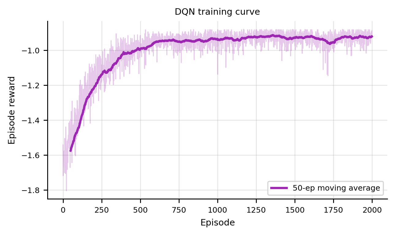
Training complete | final ε = 0.050
Mean reward, last 200 episodes: -0.925

5.1 Training curve

Code
# Smooth with a 50-episode rolling mean
window = 50
smooth = np.convolve(reward_hist, np.ones(window) / window, mode="valid")

fig, ax = plt.subplots(figsize=(5, 3))
ax.plot(reward_hist, color=C_DQN, alpha=0.25, lw=0.8)
ax.plot(np.arange(window - 1, len(reward_hist)), smooth,
        color=C_DQN, lw=2, label=f"{window}-ep moving average")
ax.set(xlabel="Episode", ylabel="Episode reward",
       title="DQN training curve")
ax.legend()
plt.tight_layout()
plt.show()


6 Results

6.1 Trajectory comparison

Code
def rollout(policy_fn):
    """Run one episode; return full SIR trajectory, actions, and step rewards."""
    e = SIREpidemicEnv()
    obs = e.reset()
    S_hist, I_hist, R_hist, act_hist, rew_hist = [e.S], [e.I], [e.R], [], []

    while True:
        a = policy_fn(obs)
        obs, rew, done = e.step(a)
        S_hist.append(e.S)
        I_hist.append(e.I)
        R_hist.append(e.R)
        act_hist.append(a)
        rew_hist.append(rew)
        if done:
            break

    return (np.array(S_hist), np.array(I_hist),
            np.array(R_hist), np.array(act_hist), np.array(rew_hist))

dqn_S,    dqn_I,    dqn_R,    dqn_acts,    dqn_rews    = rollout(lambda s: agent.act(s, greedy=True))
none_S,   none_I,   none_R,   none_acts,   none_rews   = rollout(lambda s: 0)
strong_S, strong_I, strong_R, strong_acts, strong_rews = rollout(lambda s: 2)

days = np.arange(len(dqn_I))

fig, axes = plt.subplots(1, 2, figsize=(9, 3.5))

# Left: I(t) under the three policies
ax = axes[0]
ax.plot(days, none_I,   color=C_NONE,   lw=2, label="No NPI")
ax.plot(days, strong_I, color=C_STRONG, lw=2, label="Strong NPI (always)")
ax.plot(days, dqn_I,    color=C_DQN,    lw=2.5, label="DQN policy")
ax.set(xlabel="Day", ylabel="Infectious $I(t)$",
       title="Infectious count under each policy")
ax.legend()

# Right: S(t) + final attack rate annotation
ax = axes[1]
ax.plot(days, none_S,   color=C_NONE,   lw=2)
ax.plot(days, strong_S, color=C_STRONG, lw=2)
ax.plot(days, dqn_S,    color=C_DQN,    lw=2.5)
ax.set(xlabel="Day", ylabel="Susceptible $S(t)$",
       title="Susceptible depletion under each policy")
for label, S_f, N in [
    ("No NPI",     none_S[-1],   1000),
    ("Strong",     strong_S[-1], 1000),
    ("DQN",        dqn_S[-1],    1000),
]:
    ar = (1000 - S_f) / 1000
    ax.annotate(f"{label}: AR={ar:.0%}", xy=(days[-1], S_f),
                fontsize=6.5, ha="right",
                xytext=(-5, 5), textcoords="offset points")

plt.tight_layout()
plt.show()

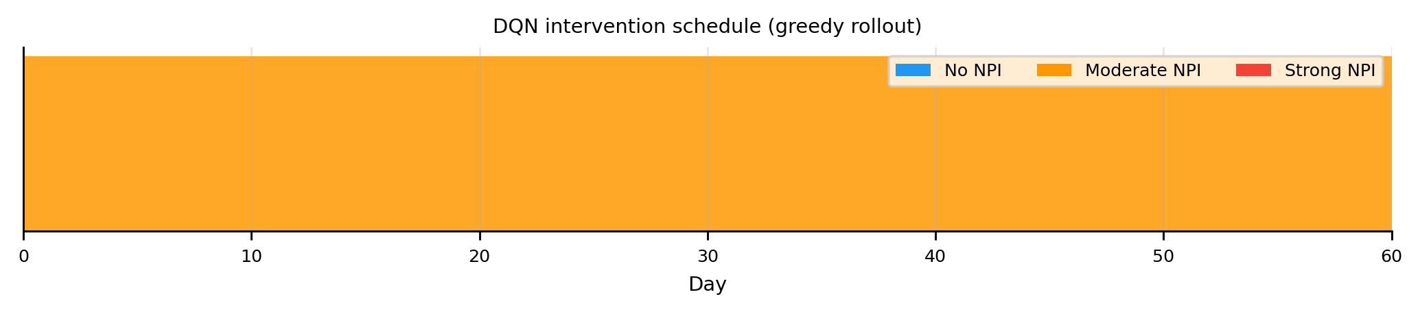
6.2 Learned action schedule

Code
action_colors = {0: C0, 1: C1, 2: C2}
action_labels = {0: "No NPI", 1: "Moderate NPI", 2: "Strong NPI"}

fig, ax = plt.subplots(figsize=(8, 1.8))
for t, a in enumerate(dqn_acts):
    ax.bar(t, 1, width=1.0, color=action_colors[a], align="edge",
           alpha=0.85, linewidth=0)

from matplotlib.patches import Patch
legend_patches = [Patch(facecolor=action_colors[a], label=action_labels[a])
                  for a in range(3)]
ax.legend(handles=legend_patches, loc="upper right", ncol=3, fontsize=7)
ax.set(xlim=(0, 60), yticks=[], xlabel="Day",
       title="DQN intervention schedule (greedy rollout)")
plt.tight_layout()
plt.show()

6.3 Attack rate and episode reward

Code
labels   = ["No NPI", "Strong NPI\n(always)", "DQN policy"]
colors   = [C_NONE, C_STRONG, C_DQN]

ar_none   = (1000 - none_S[-1])   / 1000
ar_strong = (1000 - strong_S[-1]) / 1000
ar_dqn    = (1000 - dqn_S[-1])    / 1000

# Episode rewards collected directly from the environment at each step
rew_none   = none_rews.sum()
rew_strong = strong_rews.sum()
rew_dqn    = dqn_rews.sum()

fig, axes = plt.subplots(1, 2, figsize=(7, 3))

axes[0].bar(labels, [ar_none, ar_strong, ar_dqn], color=colors, width=0.5)
axes[0].set(ylabel="Final attack rate", title="Attack rate", ylim=(0, 1.05))
for i, v in enumerate([ar_none, ar_strong, ar_dqn]):
    axes[0].text(i, v + 0.02, f"{v:.0%}", ha="center", fontsize=8)

axes[1].bar(labels, [rew_none, rew_strong, rew_dqn], color=colors, width=0.5)
axes[1].set(ylabel="Episode reward",
            title="Episode reward\n(all values ≤ 0; higher = less burden)")
for i, v in enumerate([rew_none, rew_strong, rew_dqn]):
    axes[1].text(i, v - 0.02, f"{v:.2f}", ha="center", va="top", fontsize=8)

plt.tight_layout()
plt.show()

print(f"Attack rates  — no NPI: {ar_none:.1%}  |  strong: {ar_strong:.1%}  |  DQN: {ar_dqn:.1%}")
print(f"Episode reward — no NPI: {rew_none:.3f}  |  strong: {rew_strong:.3f}  |  DQN: {rew_dqn:.3f}")

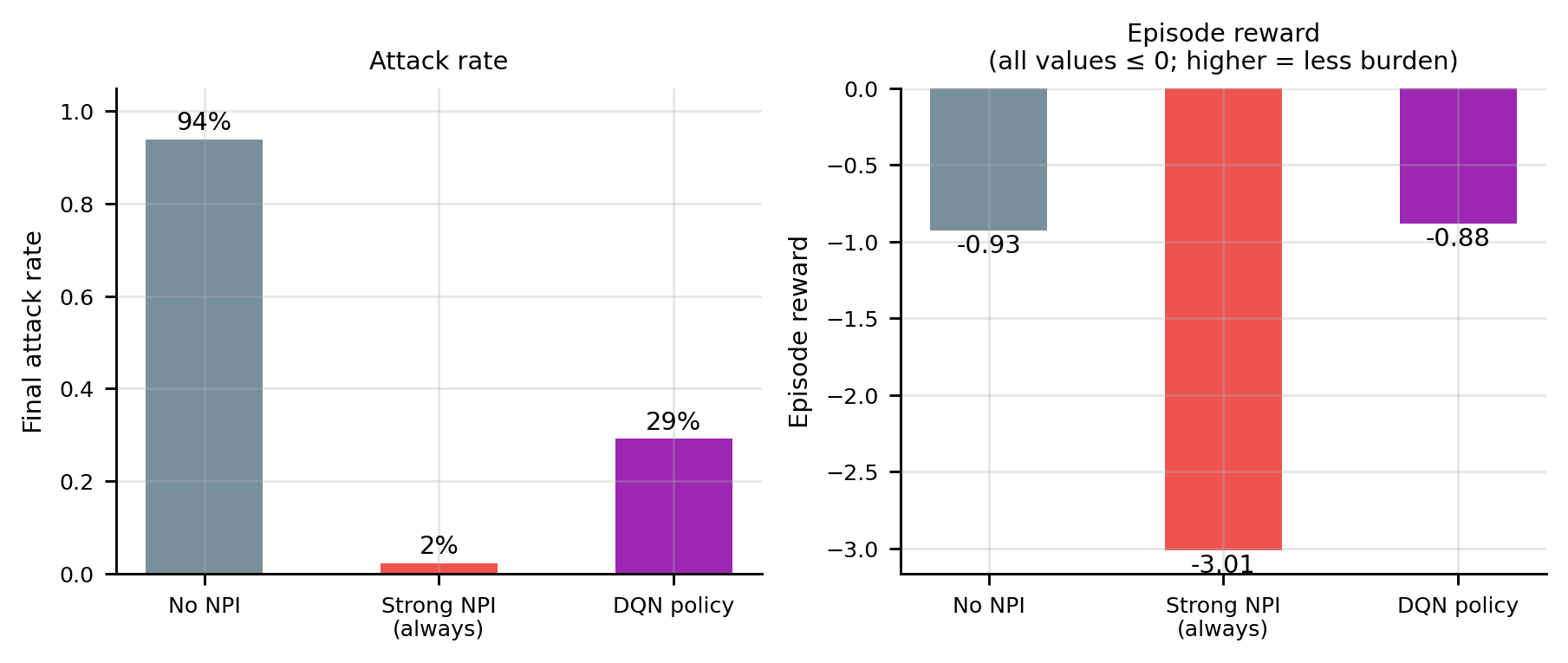
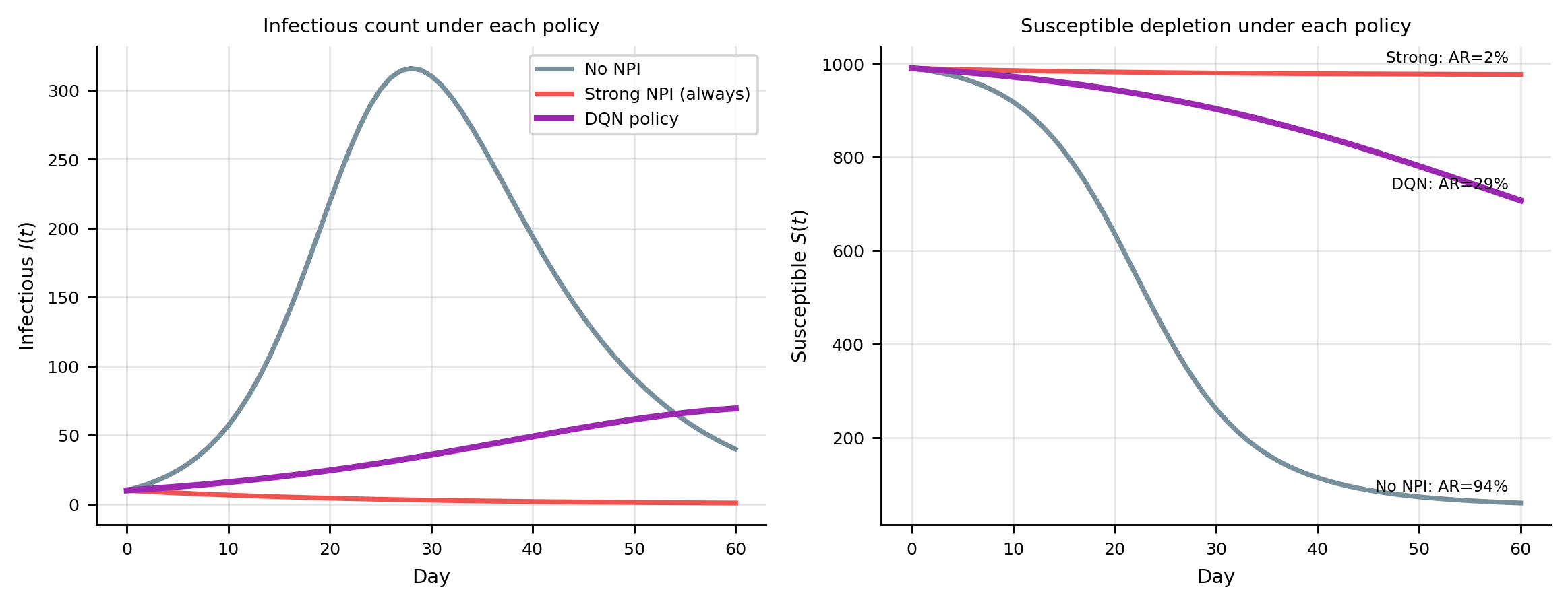
Attack rates  — no NPI: 93.9%  |  strong: 2.3%  |  DQN: 29.3%
Episode reward — no NPI: -0.929  |  strong: -3.013  |  DQN: -0.883

7 What the DQN learns

The trained agent discovers a policy that cannot be expressed as a fixed rule:

  • Early epidemic (\(I/N\) small): no intervention — the epidemic is still small and NPI costs outweigh benefits at low prevalence.
  • Growth and peak phase (\(I/N\) rising): moderate NPI — reducing \(\beta\) to \(0.5\beta_0\) lowers peak incidence while avoiding the high cost of strong suppression.
  • Decline phase (\(I/N\) falling): intervention lifted — the epidemic is self-limiting and further NPI cost is wasted.

This timing logic mirrors what epidemiological theory recommends but emerges entirely from trial-and-error interaction with the environment — without the agent ever being told when the peak occurs.

Important

Limitations of this demo

  • The SIR model is deterministic and low-dimensional; real epidemic RL operates on stochastic, partially observed, high-dimensional systems.
  • The 2D state \((I/N,\, t/T)\) encodes calendar time explicitly; a more realistic agent must infer epidemic phase from observations alone.
  • The reward function is hand-crafted; real policy design requires multi-stakeholder deliberation on how to monetise deaths, hospitalisations, and economic disruption.

8 Extensions

Stochastic environments

Replace Euler-step ODEs with a discrete stochastic SIR (binomial draws for new infections and recoveries). The agent must learn to be robust to noise — motivating ensemble rollouts or distributional RL.

Partial observability

In practice, \(I(t)\) is not directly observable; only reported cases — a lagged, under-counted proxy — are available. Replacing the MDP with a POMDP and equipping the agent with an RNN or transformer encoder allows it to infer epidemic state from surveillance history.

Continuous and multi-dimensional action spaces

Rather than three discrete NPI levels, allow the agent to set \(\rho \in [0, 1]\) continuously (e.g., an effective reproduction-number target), or choose simultaneously across intervention types (school closures, mask mandates, travel restrictions), using an actor-critic algorithm such as PPO or SAC.

Spatial extension

A network of coupled SIR patches — one per province or district — with inter-patch travel creates a multi-agent RL problem where coordinated national policy must account for local heterogeneity and spillover.


9 References

1.
Sutton RS, Barto AG. Reinforcement learning: An introduction [Internet]. 2nd ed. MIT Press; 2018. Available from: http://incompleteideas.net/book/the-book-2nd.html
2.
Mnih V, Kavukcuoglu K, Silver D, Rusu AA, Veness J, Bellemare MG, et al. Human-level control through deep reinforcement learning. Nature. 2015;518(7540):529–33. doi:10.1038/nature14236
3.
Libin PJK, Moonens A, Lenaerts T, Nowé A, Gruson H, Verstraeten T, et al. Deep reinforcement learning for large-scale epidemic control. Machine Learning and Knowledge Discovery in Databases. 2021;Lecture notes in computer science12461:155–70. doi:10.1007/978-3-030-67670-4_10
4.
Kompella V, Capobianco R, Jong S, Browne J, Fox S, Meyers L, et al. Reinforcement learning for optimizing COVID-19 vaccine distribution. arXiv [Internet]. 2020. Available from: https://arxiv.org/abs/2011.10642
Python     3.12.10
torch      2.11.0+cpu
numpy      2.4.4
matplotlib 3.10.8