Estimating serial interval for a growing epidemic

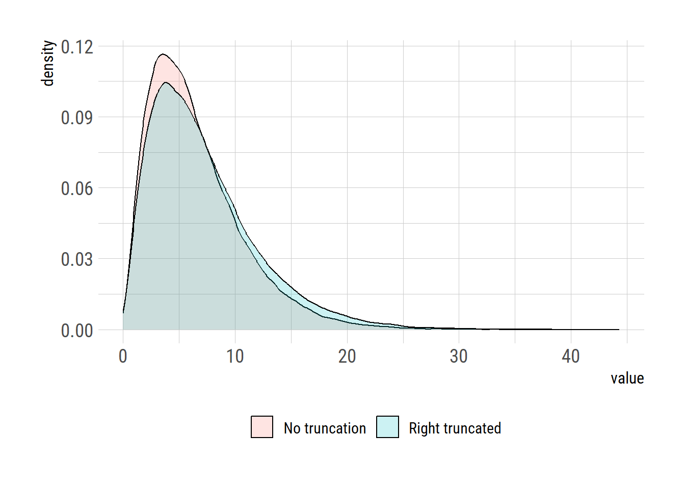
When estimating serial intervals or other time-to-event distributions from epidemic data, right truncation is a key consideration: individuals are observed only if their event time falls before some truncation time (1). The corrected likelihood accounts for this selection mechanism.

In this case, the above likelihood function may be modified as follows:

\[\mathcal{L}(X;\theta) = \prod_{i=1}^{n} f_{\theta}(B_i-A_i)\] , where \(A^L, A^R, B\) present the times for lower end and upper bound on the potential dates of symptom onset of the infector, and the symptom onset time of the infectee, respectively.

\[f^t_{\theta}(B_i-A_i) = \frac{f_{\theta}(B_i-A_i)}{F(T-A_i)}\]

set.seed(42)
n <- 1000
shape_true <- 2.2
scale_true <- 3.3

df <- data.frame(A=sample(0:30, size=n, replace=TRUE))
si <- rgamma(n, shape=shape_true, scale=scale_true)
df$B <- df$A + si
max(df$B)

[1] 57.03661

summary(df$B)

   Min. 1st Qu.  Median    Mean 3rd Qu.    Max. 
 0.3967 13.9763 22.4103 22.4031 30.3811 57.0366 

Tmax <- 35
under_Tmax <- df$B < Tmax

newdf <- df[under_Tmax,]

nll <- function(parms, A, B) -sum(dgamma(B-A, shape=parms[[1]], scale=parms[[2]], log=TRUE))
res1 = optim(par=c(1,2), fn=nll, A=newdf$A, B=newdf$B,
             method = "Nelder-Mead",
            control = list(maxit=2e4, reltol=1e-15))
res1

$par
[1] 2.366494 2.735134

$value
[1] 2389.103

$counts
function gradient 
     101       NA 

$convergence
[1] 0

$message
NULL

nll_right_trunc <- function(parms, A, B, Tmax) -sum(log(dgamma(B-A, shape=parms[[1]], scale=parms[[2]])/pgamma(Tmax-A, shape=parms[[1]], scale=parms[[2]])))

res2 = optim(par=c(1,2), 
             fn=nll_right_trunc, 
             A=newdf$A, 
             B=newdf$B,
             Tmax=Tmax,
             method = "Nelder-Mead",
             control = list(maxit=2e4, reltol=1e-15))
res2

$par
[1] 2.230993 3.230118

$value
[1] 2317.955

$counts
function gradient 
     115       NA 

$convergence
[1] 0

$message
NULL

n <- 1e5
x1 <- rgamma(n, shape=res1$par[[1]], scale=res1$par[[2]])
x2 <- rgamma(n, shape=res2$par[[1]], scale=res2$par[[2]])

summary(x1)

    Min.  1st Qu.   Median     Mean  3rd Qu.     Max. 
 0.01066  3.36629  5.58653  6.47582  8.62659 44.32536 

summary(x2)

   Min. 1st Qu.  Median    Mean 3rd Qu.    Max. 
 0.0263  3.6574  6.1697  7.2078  9.6218 43.8174 

df = data.frame(model=rep(c("No truncation", "Right truncated"), each=n), val=c(x1,x2))

library(ggplot2)
extrafont::loadfonts()
theme_set(hrbrthemes::theme_ipsum_rc(base_size=14, subtitle_size=16, axis_title_size=12))

df |> ggplot(aes(x=val, fill=model))+
  geom_density(alpha=0.2) +
  labs(x="value", y="density")+
  theme(legend.position = "bottom", 
        legend.title = element_blank())

# ggsave("right_trunc.png", gg, units="in", width=3.4*2, height=2.7*2)

References

1.

Seaman SR, Presanis AM, Jackson C. Estimating a time-to-event distribution from right-truncated data in an epidemic: A review of methods. Statistical Methods in Medical Research. 2022;31(9):1641–55. doi:10.1177/09622802211023955