Optimizing Vaccination Strategies: Preemptive vs. Reactive Vaccination

When managing infectious disease risks such as cholera, limited vaccine supply often forces decision-makers to choose between pre-emptive and reactive vaccination campaigns. This post explores a cost-benefit model comparing the two strategies using analytical expressions and numerical simulations.

We aim to answer: Under what conditions is it better to vaccinate before an outbreak occurs, and when is it more beneficial to wait and respond reactively?

1 Defining the Core Quantities

Let:

• \(B\): The full benefit gained by averting an outbreak (e.g., DALYs or cases averted)
• \(C\): The cost of deploying one vaccination campaign
• \(p\): The probability of an outbreak in a given region
• \(r\): The effectiveness of a reactive campaign one relative to pre-emptive one (e.g., \(r=0.6\) means 60% as effective)

1.1 Pre-emptive Vaccination

If we vaccinate before any outbreak, the expected benefit is \(B \cdot p\). However, we always incur the campaign cost \(C\), so the net expected benefit is:

\[ \text{Net}_{\text{pre}} = Bp - C \]

1.2 Reactive Vaccination

For reactive vaccination, the benefit is only realized if an outbreak occurs (probability \(p\)), and even then, only \(rB\) is saved due to delays. The cost \(C\) is only paid if an outbreak occurs. Hence:

\[ \text{Net}_{\text{react}} = Bpr - Cp \]

2 Comparison of two strategies

\[ \text{Net}_{\text{pre}} - \text{Net}_{\text{react}} = pB(1 - r) - C(1 - p) \]

2.1 Interpretation

Pre-emptive is better if:

\[ pB(1 - r) > C(1 - p) \]

Solving for \(p\) gives the threshold outbreak probability \(p^*\):

Code

import sympy as sp

# Define symbols
B, C, p, r = sp.symbols('B C p r', positive=True)

# Net benefits
net_pre   = B*p - C
net_react = B*p*r - C*p

# When is pre-emptive better?
threshold_p = sp.solve(net_pre - net_react > 0, p)

\[ p > \frac{C}{B(1 - r) + C} \]

3 Visualizing the Break-even Probability

Code

library(ggplot2)
library(dplyr)

# Create a grid of r and p values
r_vals <- seq(0.1, 0.9, by = 0.01)
p_vals <- seq(0.01, 0.99, by = 0.01)
B <- 1
C <- 0.4

# Compute threshold for each r
grid <- expand.grid(p = p_vals, r = r_vals)
grid <- grid %>%
  mutate(p_star = C / (B * (1 - r) + C),
         decision = ifelse(p > p_star, "Preemptive", "Reactive"))

# Plot heatmap
ggplot(grid, aes(x = r, y = p, fill = decision)) +
  geom_tile(color = "white") +
  scale_fill_manual(values = c("Preemptive" = "steelblue", "Reactive" = "tomato")) +
  labs(title = "Vaccination Strategy Decision Heatmap",
       x = "Relative Reactive Benefit (r)",
       y = "Outbreak Probability (p)",
       fill = "Strategy") +
  theme_minimal()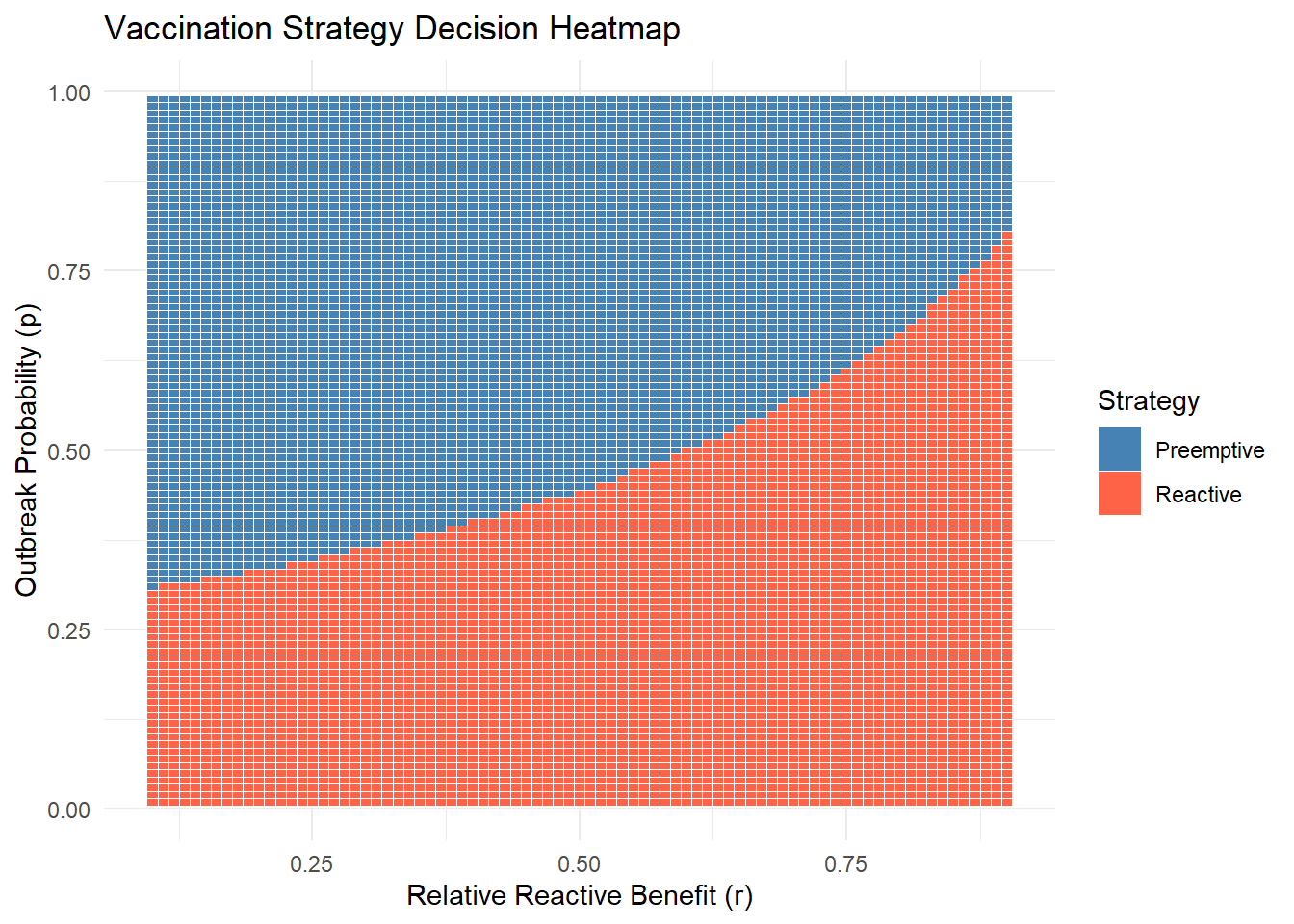

This plot shows that reactive vaccination is better when \(p\) is small, but pre-emptive takes over beyond a break-even point that depends on \(r\).

4 dditional benefits of pre-emptive vaccination and the cost of using deploying vaccines

We define two additional parameters - \(\phi\): The benefit of vaccination when no outbreak occurs (e.g., due to future immunity or prevention). This applies to both pre-emptive and reactive strategies

• \(D\): The cost or penalty associated with unused reactive vaccines (e.g., due to expiry or logistical waste)

4.1 Pre-emptive Vaccination

If we vaccinate before any outbreak, the expected benefit includes two parts:

• \(pB\) when an outbreak is averted
• \((1 - p)\phi B\) when no outbreak occurs but future benefit remains

The cost \(C\) is always incurred. So the net expected benefit is:

\[ \text{Net}_{\text{pre}} = pB + (1 - p)\phi B - C \]

4.2 Reactive Vaccination

Reactive benefit occurs only if an outbreak occurs. In that case:

• Benefit: \(rB\) and \(\phi B\) with probability \(p\)
• Cost: \(C\) with probability \(p\)
• Penalty (waste): \(D\) with probability \((1 - p)\)

So the net expected benefit is:

\[ \text{Net}_{\text{react}} = p(r+\phi)B - pC - (1 - p)D \]

Compare symbolically both strategies under these extended conditions.

Code

import sympy as sp

# Define symbols
B, C, D, p, r, phi = sp.symbols('B C D p r phi', positive=True)

# Net benefits
net_pre   = p*B + (1 - p)*phi*B - C
net_react = p*(r+phi)*B - p*C - (1 - p)*D

# Difference
diff = net_pre - net_react
sp.simplify(diff)

-B*p*(phi + r) + B*p - B*phi*(p - 1) + C*p - C - D*(p - 1)

Code

threshold_p = sp.solve(diff > 0, p)

\[ \text{Net}_{\text{pre}} - \text{Net}_{\text{react}} = Bp(1 - r - \phi) + B(1 - p)\phi - C(1 - p) + D(1 - p) \]

Pre-emptive vaccination is better when this expression is positive. The threshold for \(p\) can be derived numerically based on values of \(B, C, D, r, \phi\).

5 Visualizing the Extended Model

We update the R plot to incorporate \(\phi\) and \(D\).

Code

library(ggplot2)
library(dplyr)

B <- 1
C <- 0.5
D <- 0.02
phi <- 0.1
r_vals <- seq(0.1, 0.9, by = 0.01)
p_vals <- seq(0.01, 0.99, by = 0.01)

compute_net <- function(p, r) {
  net_pre   <- B * p + (1 - p) * B * phi - C
  net_react <- B * p * (r + phi)  - p * C - (1 - p) * D
  return(data.frame(p = p, r = r,
                    net_pre = net_pre,
                    net_react = net_react))
}

# Compute threshold for each r
grid <- expand.grid(p = p_vals, r = r_vals)
grid <- grid %>% 
  mutate(pre = compute_net(p,r)$net_pre,
         react = compute_net(p,r)$net_react,
         decision = ifelse(pre > react, "Preemptive", "Reactive"))

# Plot heatmap
ggplot(grid, aes(x = r, y = p, fill = decision)) +
  geom_tile(color = "white") +
  scale_fill_manual(values = c("Preemptive" = "steelblue", "Reactive" = "tomato")) +
  labs(title = "Vaccination Strategy Decision Heatmap",
       x = "Relative Reactive Benefit (r)",
       y = "Outbreak Probability (p)",
       fill = "Strategy") +
  theme_minimal()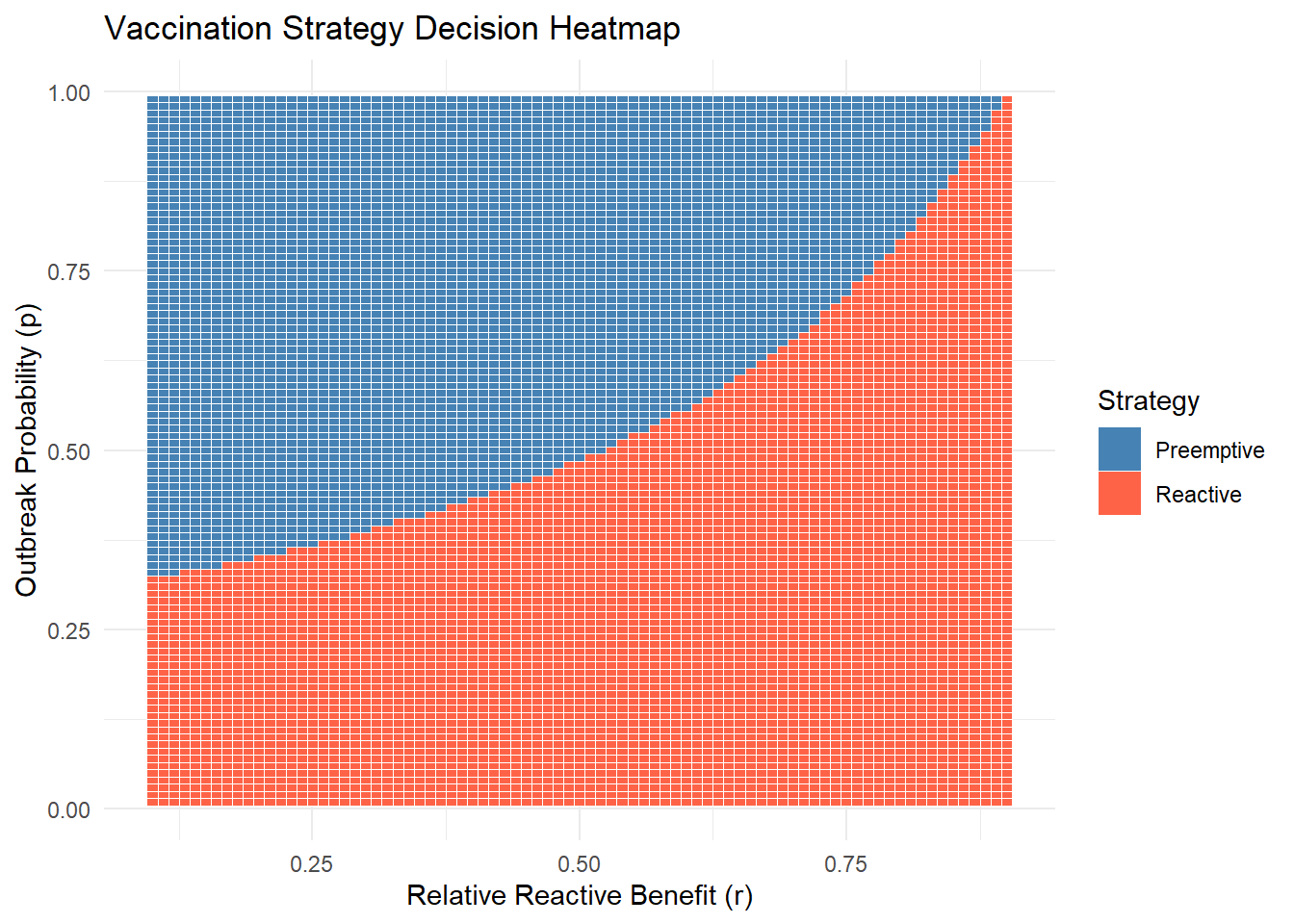

6 Interpretation

7 Extending to Multiple Sub-populations

Let’s now generalize to \(k\) sub-populations, each with its own outbreak probability \(p_i\). We have \(m\) campaigns to deploy:

• Assign \(m_{\text{pre}}\) campaigns pre-emptively
• Leave \(m_{\text{react}} = m - m_{\text{pre}}\) campaigns for reactive use

7.1 Strategy:

• Sort sub-populations by descending \(p_i\)
• Pre-emptively vaccinate top \(m\_{\text{pre}}\) if \(p_i > \frac{- \phi B+ C - D}{(1- 2 \phi - r)B + C - D}\)
• Use remaining campaigns reactively

This is equivalent to choosing all sub-populations where:

\[ p_i > \frac{- \phi B+ C - D}{(1- 2 \phi - r)B + C - D} \]

---

8 Numerical illustration in R

We simulate 10 sub-populations with different outbreak probabilities and show how many campaigns should be used pre-emptively.

Code

set.seed(42)
p_i <- sort(runif(10, 0.05, 0.6), decreasing = TRUE)
threshold_p <- function(B, C, r) { C / (B * (1 - r) + C) }

assign_campaigns <- function(p_i, B, C, r) {
  p_star <- threshold_p(B, C, r)
  preemptive <- which(p_i > p_star)
  data.frame(index = 1:length(p_i), p_i = p_i,
             decision = ifelse(p_i > p_star, "pre-emptive", "reactive"))
}

assign_campaigns(p_i, B = 1, C = 0.2, r = 0.6)

   index       p_i    decision
1      1 0.5653915 pre-emptive
2      2 0.5531433 pre-emptive
3      3 0.5067462 pre-emptive
4      4 0.4551236 pre-emptive
5      5 0.4377856 pre-emptive
6      6 0.4113458 pre-emptive
7      7 0.4029600 pre-emptive
8      8 0.3355028 pre-emptive
9      9 0.2073767    reactive
10    10 0.1240666    reactive

9 Further extention:

We consider a strategic vaccination scenario where oral cholera vaccines (OCVs) are in limited supply. Specifically, the available stockpile is sufficient to cover only 10% of all subpopulations. Epidemiological data suggest that, within the anticipated time frame, fewer than 10% of subpopulations are likely to experience an outbreak. This implies that a fully reactive strategy—in which vaccines are deployed only in response to confirmed outbreaks—could, in principle, respond to all outbreaks without exceeding supply.

However, a recent risk assessment indicates that 20% of the population exceeds the outbreak probability threshold \(p^*\) above which preemptive vaccination is expected to yield greater benefit than reactive vaccination for a given region.

This raises a strategic dilemma:

Should all subpopulations above the preemptive threshold be vaccinated in advance, despite limited vaccine availability and the potential need for reactive response elsewhere?

This scenario highlights the trade-off between targeting high-risk areas proactively versus preserving flexibility to respond where outbreaks actually occur, especially under uncertainty and supply constraints. That is, we need to consider an opportunity cost of preemptive vaccination under Limited vaccine supply.

10 Setting and Assumptions

• \(n\): total number of subpopulations.
• \(M\): number of vaccine campaigns available.
• \(k\): number of regions chosen for preemptive vaccination.
• \(p_i\): outbreak probability in region \(i\), with $p_1 p_2 p_n $.

Assumptions: - You can identify top-\(k\) highest-risk regions. - You can react to up to \(M - k\) outbreaks in unvaccinated populations. - Outbreaks occur independently across regions.

---

11 1. Expected Benefit: Preemptive Strategy

Vaccinate top \(k\) high-risk regions:

\[\text{Benefit}_{\text{pre}} = \sum_{i=1}^{k} p_i B \]

---

12 2. Expected Benefit: Reactive Strategy

Let $ k = {i=k+1}^{n} p_i $: expected number of outbreaks in unvaccinated regions.

Expected reactive benefit (up to $ M - k $ responses):

\[ \text{Benefit}_{\text{react}} = rB \cdot \min(M - k, \mu_k) \]

---

13 3. Total Expected Benefit

\[ \text{Total Benefit}_k \approx B \left( \sum_{i=1}^{k} p_i + r \cdot \min(M - k, \mu_k) \right) \]

---

14 4. Opportunity Cost of Preemptive Vaccination

Vaccinating region \(k+1\) preemptively: - Gain: \(p_{k+1} B\) - Lose: ability to respond reactively to one more outbreak

Opportunity cost:

\[ \text{Opportunity Cost}(k+1) = rB \cdot \mathbb{P}(X_k \ge M - k) \]

where \(X_k \sim \text{Binomial}(n - k, \bar{p}_k)\) or $(_k) $.

---

15 5. Refined Decision Rule

Preemptively vaccinate region \(i\) only if:

\[ p_i > r \cdot \mathbb{P}(\text{reactive demand exceeds remaining doses}) \]

Using Poisson approximation:

\[ \mathbb{P}(X_k \ge M - k) \approx 1 - \sum_{x=0}^{M-k-1} \frac{e^{-\mu_k} \mu_k^x}{x!} \]

So:

\[ \text{Opportunity Cost} \approx rB \left(1 - \sum_{x=0}^{M-k-1} \frac{e^{-\mu_k} \mu_k^x}{x!} \right) \]

---

16 Summary of Key Formulas

Quantity	Expression
Preemptive threshold	$ p^* = $
Preemptive benefit (k regions)	$_{i=1}^k p_i B $
Reactive expected benefit	$ rB (M-k, _k) $
Total expected benefit	$ B ( _{i=1}^k p_i + r (M - k, _k) ) $
Opportunity cost of dose $ k+1 $	$ rB (X_k M - k) $
Adjusted decision rule	Vaccinate if $ p_{k+1} > r (X_k M - k) $

---

Code

# Load necessary libraries
library(ggplot2)
library(dplyr)

# Simulation parameters
set.seed(123)
n <- 100                        # Total subpopulations
M <- 10                         # Vaccine budget (10% of regions)
B <- 1                          # Benefit of preventing an outbreak
C <- 0.4                        # Cost of vaccination
r <- 0.8                        # Relative reactive benefit
phi <- 0.05
D <- 0.1

# Threshold for preemptive action
p_star <- (- phi*B + C - D) / ((1- 2*phi - r)*B + C - D)
# p_star <- C / (B * (1 - r) + C) 

# Generate synthetic outbreak probabilities
p_i <- sort(runif(n, 0.01, 0.5), decreasing = TRUE)

# Simulate outbreak events (Bernoulli trial based on p_i)
n_sim <- 1000
results <- data.frame()

for (k in 0:M) {
  # Preemptively vaccinate top-k at-risk regions
  preempt_indices <- 1:k
  reactive_pool <- (k+1):n

  total_cases_averted <- numeric(n_sim)

  for (s in 1:n_sim) {
    outbreaks <- rbinom(n, 1, p_i)

    # Preemptive: full benefit if outbreak occurs
    preempt_impact <- sum(outbreaks[preempt_indices]) * B

    # Reactive: respond to up to (M - k) actual outbreaks in unvaccinated group
    reactive_indices <- reactive_pool[outbreaks[reactive_pool] == 1]
    max_reactive <- min(length(reactive_indices), M - k)
    reactive_impact <- max_reactive * r * B

    total_cases_averted[s] <- preempt_impact + reactive_impact
  }

  results <- rbind(results,
                   data.frame(
                     k_preempt = k,
                     mean_cases_averted = mean(total_cases_averted),
                     sd = sd(total_cases_averted)
                   ))
}

# Plot
ggplot(results, aes(x = k_preempt, y = mean_cases_averted)) +
  geom_line(size = 1.2) +
  geom_ribbon(aes(ymin = mean_cases_averted - sd,
                  ymax = mean_cases_averted + sd),
              fill = "skyblue", alpha = 0.3) +
  labs(title = "Expected Cases Averted vs. Number of Preemptive Vaccinations",
       x = "Number of Preemptive Vaccinated Regions (k)",
       y = "Mean Cases Averted (with SD band)") +
  theme_minimal()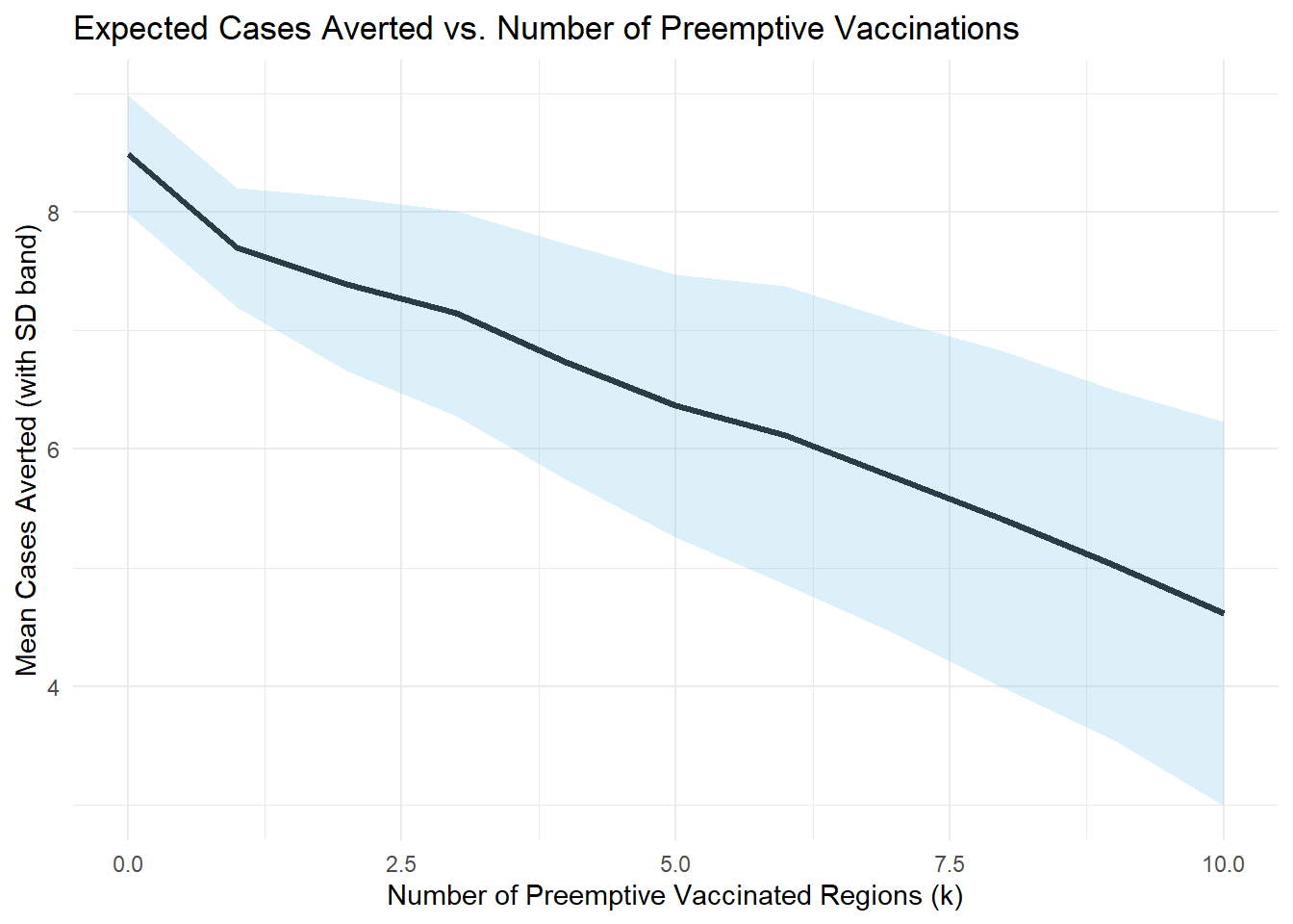

17 Discussion

When outbreak risk is high enough, pre-emptive vaccination pays off even if the outbreak doesn’t occur. When outbreak risk is low, and reactive campaigns are effective (\(r\) close to 1) and is more cost-effective. The decision threshold depends critically on the relative cost \(C\) and the delay penalty \((1 - r)\) in addition to \(p\) and \(r\)

18 Conclusion

Even under limited vaccine supply, careful cost-benefit modeling can guide whether to vaccinate early or wait. This blog post outlined a tractable analytical framework and practical tools (in Python and R) to support such decisions. Extensions could include waning immunity, spatial correlations, or dynamic outbreaks.