To Wait or To Act? Optimizing Reactive vs. Pre-emptive Vaccination Strategies

1 Background

Preventing and controlling infectious disease outbreaks requires making strategic use of limited vaccine stockpiles. This challenge is especially acute for diseases such as cholera and typhoid fever, where global supplies remain constrained and timely deployment is crucial. In principle, directing vaccines toward high-risk populations should yield the greatest benefit, but real-world uncertainty—in outbreak timing, risk signals, and operational response—can make simple pro-rata allocation surprisingly competitive.

Existing modeling studies typically assume that outbreaks will occur in a given time horizon and evaluate strategies only conditional on an epidemic happening. What remains unclear is how to choose between pre-emptive, reactive, or mixed vaccination strategies when outbreaks are uncertain and when economic constraints matter.

To address this gap, we developed a general analytical framework that identifies the vaccination strategy minimizing total expected societal cost, including both vaccination expenditures and potential outbreak losses. Our approach integrates limited vaccine supply, heterogeneous outbreak risks, targeting accuracy, and economic trade-offs.

Using closed-form analytical results, we characterize optimal allocation rules across a range of operational settings. This framework provides practical, quantitative guidance for policymakers designing vaccination strategies under uncertainty.

2 Key Existing Studies

1. Azman and Lessler (2015): Investigated reactive vaccination against cholera with limited supply. They found that optimal allocation depends on connectivity, transmission efficiency, timing, and availability. In highly connected settings, targeting hotspots is only optimal if done very early; otherwise, broader distribution is preferred.

2. Klepac, Laxminarayan, and Grenfell (2011): Analyzed pre-emptive strategies under economic constraints. They showed that optimal coverage is determined by the ratio of disease burden to vaccination costs, independent of \(\mathcal{R}_0\). For coupled populations, local optima often conflict with global goals, necessitating coordination.

Insight from 1 & 2: Strong regional coupling requires looking beyond the initial outbreak site, though these models often overlook delays in detection.

3. Klepac, Bjørnstad, et al. (2012): Examined the trade-off between reactive vaccination and palliative care under a fixed budget. The optimal switch point depends on relative costs and \(\mathcal{R}_0\). For highly transmissible diseases, the window for vaccination is narrow, making palliative care optimal even before the epidemic peak.

Insight from 1, 2, & 3: High \(\mathcal{R}_0\) pathogens leave a very short window for intervention, often requiring a shift to alternative strategies or targeting connected regions.

4. Matrajt, Halloran, and Longini (2013): Studied reactive vaccination for pandemic influenza. Cooperative allocation significantly outperforms pro-rata distribution, but effectiveness requires extremely fast implementation (within the first few weeks).

5. Keeling and White (2011): Focused on logistical constraints during pandemic influenza. They found that starting early is more beneficial than vaccinating quickly. In realistic scenarios, targeting high-risk groups is generally superior to targeting high-transmission groups.

6. Wu, Riley, and Leung (2007): Evaluated pre-emptive geographic allocation for influenza. While pro-rata allocation is the least efficient, the marginal gains from prioritization are often small and sensitive to uncertainty. Thus, pro-rata remains a robust compromise for equity and simplicity.

7. Keeling and Shattock (2012): Explored pre-emptive vaccination in isolated vs. coupled populations. To minimize final size with limited supply, the optimal policy is often highly inequitable (targeting small populations for herd immunity), though coupling pushes the strategy toward a more uniform distribution.

8. Wallinga, van Boven, and Lipsitch (2010): Proposed a robust principle for scarce control measures: prioritize groups with the highest product of incidence and force of infection. For social distancing, priority should be proportional to the square of infection incidence.

3 Economic costs of outbreaks and vaccination campaign

3.1 Cost of an outbreak

1. Direct medical costs

This component covers the cost of inpatient and outpatient care for all cholera cases:

\[ C_{\text{illness}}^{\text{direct}} = N_{\text{inpatient}}\times C_{\text{inpatient}} + N_{\text{outpatient}}\times C_{\text{outpatient}} . \]

2. Productivity loss due to illness

We estimate:

\[ C_{\text{illness}}^{\text{indirect}}= N_{\text{cases}}\times d \times w, \]

where

• \(d\): average number of workdays lost per case
• \(w\): average daily wage

3. Productivity loss due to premature death

We compare two approaches:

• Approach 1: Human Capital (Present Value of Lost Income)

\[ C_{\text{death}}^{\text{HC}} = D \times \sum_{t=1}^{YLL} \frac{G}{(1+\delta)^t} \]

• Approach 2: Value of Statistical Life (VSL)

\[ C_{\text{death}}^{VSL} = D \times V \]

Where:

• \(D\): number of deaths
• \(YLL\): average years of productive life lost
• \(G\): GDP per capita
• \(\delta\): discount rate (e.g., 0.03)
• \(V\): estimated value of statistical life (in USD)

The total outbreak cost or the cost from infection is

\[ C_{\text{outbreak}} = C_I = C_{\text{illness}}^{\text{direct}} + C_{\text{illness}}^{\text{indirect}} + C_{\text{death}}. \]

3.2 Cost of a cholera vaccination program

We use:

\[ C_{\text{vaccination}} = C_V =N_{\text{people}}\times (c_{\text{dose}} + c_{\text{delivery}}), \]

where \(c_{\text{dose}}\) and \(c_{\text{delivery}}\) denote vaccine cost per dose and delivery cost per dose, respectively.

4 Scenarios

Let:

• \(p_i\) = outbreak probability for population \(i\), \(i = 1,\dots,n\),
• \(C_I\) = outbreak cost arising from infections,
• \(C_V\) = vaccination cost,
• \(\nu \in [0,1]\) = effectiveness of pre-emptive vaccination,
• \(r \in [0,1]\) = effectiveness of reactive vaccination,
• \(R = C_I/C_V\) = outbreak–to–vaccination cost ratio,
• \(f \in (0,1]\) = total vaccination capacity as a fraction of populations,
• \(\alpha \in [0,1]\) = fraction of vaccination capacity used pre-emptively,
• \(f_{\mathrm{pre}} = \alpha f\) = fraction of populations vaccinated pre-emptively,
• \(f_{\mathrm{react}} = (1-\alpha)f\) = vaccination capacity reserved for reactive campaigns.

4.1 One Population

We consider a single population with outbreak probability \(p\), outbreak cost \(C_I\), vaccination cost \(C_V\), pre-emptive vaccination effectiveness \(\nu \in [0,1]\), and reactive vaccination effectiveness \(r \in [0,1]\). The outbreak cost \(C_I\) reflects direct medical costs, productivity losses, and mortality-related losses. The vaccination cost \(C_V\) includes vaccine and delivery costs.

Let \(X \sim \mathrm{Bernoulli}(p)\) denote an indicator of an outbreak, where \(X=1\) if an outbreak occurs and \(X=0\) otherwise.

4.1.1 Pre-emptive strategy

Under pre-emptive vaccination, the population is vaccinated regardless of whether an outbreak occurs. Outbreak cost is \((1-\nu) C_I\) if an outbreak occurs, and \(0\) otherwise. So the total cost random variable is:

\[ C_{\mathrm{pre}}(X) = C_V + (1-\nu) X C_I. \]

Taking expectation,

\[ \mathbb{E}[C_{\mathrm{pre}}] = C_V + p (1-\nu) C_I. \]

4.1.2 Reactive strategy

Under reactive vaccination, the population is vaccinated only if an outbreak occurs. If \(X=1\), the vaccination cost \(C_V\) is incurred and residual outbreak costs equal \((1-r) C_I\). If \(X=0\), there is no cost. The total cost random variable is:

\[ C_{\mathrm{react}}(X) = X\bigl(C_V + (1-r)C_I\bigr). \]

Taking expectation,

\[ \mathbb{E}[C_{\mathrm{react}}] = p\bigl(C_V + (1-r)C_I\bigr). \]

This calculation assumes no penalty or loss from unused vaccine stock. In practice, vaccine expiry may incur additional costs, but these are omitted here for analytical clarity.

4.1.3 Normalized Per-Population Expected Costs

Define the outbreak-to-vaccination cost ratio:

\[ R = \frac{C_I}{C_V}. \]

Normalizing by \(C_V\):

4.1.3.1 Pre-emptive:

\[ c_{\mathrm{pre}}^{(1)} = \frac{\mathbb{E}[C_{\mathrm{pre}}]}{C_V} = 1 + p(1-\nu)R. \]

4.1.3.2 Reactive:

\[ c_{\mathrm{react}}^{(1)} = \frac{\mathbb{E}[C_{\mathrm{react}}]}{C_V} = p\bigl[1 + (1-r)R\bigr]. \]

These represent the normalized per-population expected costs of the two strategies with the superscript \((1)\) indicating one-population case.

Code

# --- Parameters for the illustration ---
p_vals <- seq(0, 1, 0.01) # mean outbreak probability
R_vals <- c(5)
r_vals <- c(0.3, 0.7)
nu_val <- 0.9

df_cost <- expand.grid(
    p = p_vals,
    r = r_vals,
    R = R_vals
) |>
    dplyr::mutate(
        c_pre   = cost_pre_one(p, R, r, nu = nu_val),
        c_react = cost_react_one(p, R, r, nu = nu_val),
        r_label = paste0("italic(r)==", r)
    ) |>
    tidyr::pivot_longer(
        cols      = c(c_pre, c_react),
        names_to  = "strategy",
        values_to = "cost"
    ) |>
    dplyr::mutate(
        strategy = factor(
            strategy,
            levels = c("c_pre", "c_react"),
            labels = c(paste0("Pre-emptive (\u03bd=", nu_val, ")"), "Reactive")
        )
    )

# threshold probability
# df_pstar <- expand.grid(r = r_vals, R = R_vals) |>
#   dplyr::mutate(
#     p_star  = p_star_one(R, r),
#     r_label = paste0("r = ", r)
#   )
df_pstar <- expand.grid(r = r_vals, R = R_vals) |>
    dplyr::mutate(
        p_star = p_star_one(R, r, nu = nu_val),
        r_label = paste0("r = ", r),

        # [NEW] Create the dynamic label string here
        # ~ adds a space, italic(r)==r adds the value
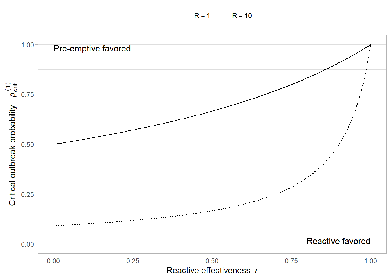
        label_expr = paste0("italic(p)[crit]^(1) ~ (italic(r) == ", r, ")")
    )

# data for braces
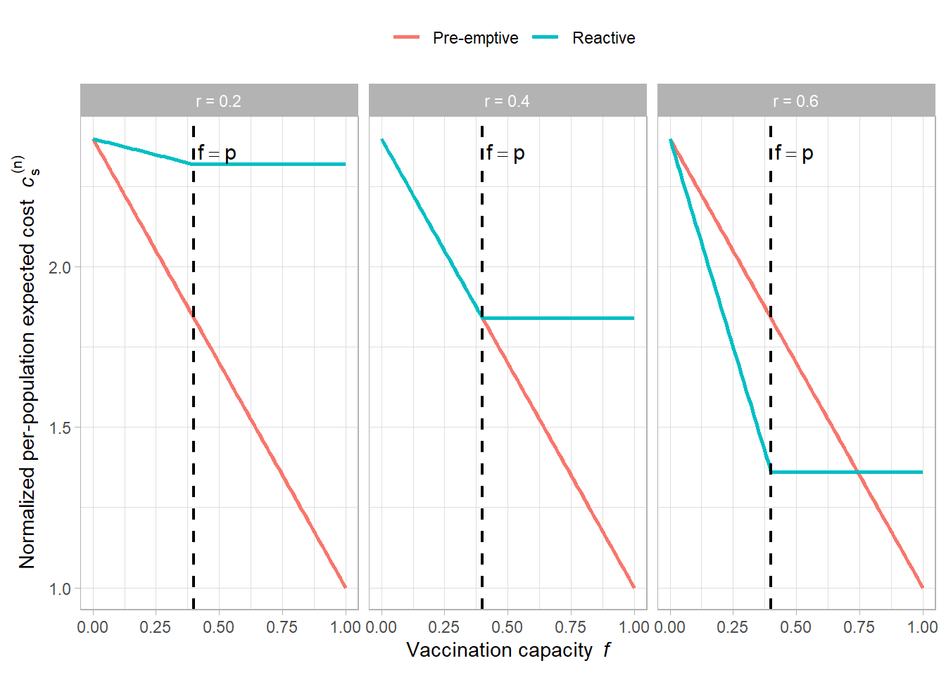
cost_preempt_max <- max(filter(df_cost, strategy == paste0("Pre-emptive (\u03bd=", nu_val, ")"), r_label == "italic(r)==0.3")$cost)
cost_react_max1 <- max(filter(df_cost, strategy == "Reactive", r_label == "italic(r)==0.7")$cost)
cost_react_max2 <- max(filter(df_cost, strategy == "Reactive", r_label == "italic(r)==0.3")$cost)

df_brace1 <- data.frame(x = c(0.96, 1), y = c(cost_preempt_max, cost_react_max1))
df_brace2 <- data.frame(x = c(0.97, 1), y = c(cost_preempt_max, cost_react_max2))
df_brace3 <- data.frame(x = c(0, 0.03), y = c(0, 1))

# convenient variables for the overhead-cost text position
text_overhead_x <- max(df_brace3$x) + 0.01 # 0.04
text_overhead_y <- mean(df_brace3$y) + 1 # 1.5
annot_text_size <- 4

ggplot(df_cost, aes(
    x = p, y = cost, color = strategy,
    linetype = r_label
)) +
    geom_line(linewidth = 1) +
    geom_vline(
        data = df_pstar,
        aes(xintercept = p_star),
        linetype = "dashed",
        color = "firebrick"
    ) +
    geom_text(
        data = df_pstar,
        aes(x = p_star, y = Inf, label = label_expr),
        parse = TRUE,
        inherit.aes = FALSE,
        hjust = -0.03,
        vjust = 1.1,
        size = 4
    ) +
    ggbrace::stat_brace(
        data = df_brace1,
        mapping = aes(x, y),
        outside = FALSE, rotate = 270,
        linewidth = 1, inherit.aes = FALSE
    ) +
    annotate("text",
        x = min(df_brace1$x) - 0.01,
        y = mean(df_brace1$y),
        label = "Cost of delayed\nresponse (r=0.7)",
        hjust = 1, size = annot_text_size, lineheight = 0.9
    ) +
    ggbrace::stat_brace(
        data = df_brace2,
        mapping = aes(x, y),
        outside = FALSE, rotate = 270,
        linewidth = 1, inherit.aes = FALSE
    ) +
    annotate("text",
        x = min(df_brace2$x) - 0.01, y = mean(df_brace2$y),
        label = "Cost of delayed\nresponse (r=0.3)",
        hjust = 1, size = annot_text_size, lineheight = 0.9
    ) +
    ggbrace::stat_brace(
        data = df_brace3,
        mapping = aes(x, y),
        outside = FALSE, rotate = 90,
        linewidth = 1, inherit.aes = FALSE
    ) +
    annotate("text",
        x = max(df_brace3$x) + 0.01,
        y = mean(df_brace3$y) + 1,
        label = "Vaccination cost",
        hjust = 0, size = annot_text_size, lineheight = 0.9
    ) +
    annotate("segment",
        x = text_overhead_x + 0.03,
        y = text_overhead_y - 0.1,
        xend = 0.02, yend = 0.75,
        arrow = arrow(length = grid::unit(0.15, "cm")),
        colour = "black"
    ) +
    scale_color_manual("", values = c("firebrick", "steelblue")) +
    scale_linetype_discrete(labels = scales::label_parse()) +
    labs(
        x = expression("Probability of an outbreak " ~ italic(p)),
        y = expression("Normalized per-population expected cost  " ~ italic(c)[s]^"(1)"),
        color = "",
        linetype = ""
    ) +
    theme_light() +
    theme(legend.position = "top") +
    guides(
        linetype = guide_legend(
            override.aes = list(color = "steelblue")
        )
    )

4.1.4 Critical Outbreak Probability \(p_{\mathrm{crit}}^{(1)}\)

The critical outbreak probability \(p_{\mathrm{crit}}^{(1)}\) at which the two strategies yield equal expected cost is given by:

\[ c_{\mathrm{pre}}^{(1)} = c_{\mathrm{react}}^{(1)} \quad\Longrightarrow\quad 1 + p(1-\nu)R = p[1 + (1-r)R] \]

\[ \quad\Longrightarrow\quad 1 = p[1 + R(\nu - r)] \quad\Longrightarrow\quad p_{\mathrm{crit}}^{(1)} = \frac{1}{1 + R(\nu - r)}. \]

• Pre-emptive preferred when \[ p > p_{\mathrm{crit}}^{(1)} \quad\Longleftrightarrow\quad c_{\mathrm{pre}}^{(1)} < c_{\mathrm{react}}^{(1)}. \]

• Reactive preferred when \[ p < p_{\mathrm{crit}}^{(1)} \quad\Longleftrightarrow\quad c_{\mathrm{pre}}^{(1)} > c_{\mathrm{react}}^{(1)}. \]

• Indifference point \[ p = p_{\mathrm{crit}}^{(1)} \quad\Longleftrightarrow\quad c_{\mathrm{pre}}^{(1)} = c_{\mathrm{react}}^{(1)}. \]

The critical probability \(p_{\mathrm{crit}}^{(1)}\) decreases as the outbreak cost ratio \(R\) increases, the pre-emptive effectiveness \(\nu\) increases, or the reactive effectiveness \(r\) decreases. Consequently, pre-emptive vaccination becomes more favorable when outbreaks are relatively more costly or when the effectiveness gap \(\nu - r\) between pre-emptive and reactive vaccination widens.

4.1.4.1 Phase diagram of \(p\) vs \(r\) for \(R=1\) and \(R=10\).

Lines in the plot represent the critical outbreak probability, \(p_{\mathrm{crit}}^{(1)}\), for the respective cost ratio \(R\).

Code

p_vals <- seq(0, 1, 0.01) # mean outbreak probability
R_vals <- c(1, 10)
r_vals <- seq(0, 1, 0.01)

data <- expand.grid(r = r_vals, R = R_vals) %>%
    dplyr::mutate(
        pstar = p_star_one(R = R, r = r, nu = 1),
        R_label = factor(
            R,
            levels = c(1, 10),
            labels = c("R = 1", "R = 10")
        )
    )
# LaTeX labels for xdvir::geom_latex()
eq_labels <- c(
    "$c_{\\text{pre}}^{(1)} < c_{\\text{react}}^{(1)}$",
    "$c_{\\text{pre}}^{(1)} > c_{\\text{react}}^{(1)}$"
)

pcrit_labels <- c(
    "$p_{\\text{crit}}^{(1)}(R=1)$",
    "$p_{\\text{crit}}^{(1)}(R=10)$"
)

plt <- ggplot(data, aes(x = r, y = pstar, linetype = R_label)) +
    geom_line() +
    # geom_abline(
    #   slope = 1, intercept = 0,
    #   linetype = "dotted",
    #   linewidth = 1,
    #   color = "firebrick"
    # ) +
    labs(
        x = expression("Reactive effectiveness " ~ italic(r)),
        y = expression("Critical outbreak probability  " ~ italic(p)[crit]^(1))
    ) +
    theme_light() +
    theme(legend.position = "top") +
    # Existing text labels
    annotate("text",
        size = 4, x = 0, y = 1,
        hjust = 0, vjust = 1,
        label = "Pre-emptive favored"
    ) +
    annotate("text",
        size = 4, x = 1, y = 0,
        hjust = 1, vjust = 0,
        label = "Reactive favored"
    ) +
    annotate(
        "latex",
        x = 0, y = 0.93,
        label = eq_labels[1],
        size = 4, hjust = 0, vjust = 1
    ) +
    annotate(
        "latex",
        x = 1, y = 0.07,
        label = eq_labels[2],
        size = 4, hjust = 1, vjust = 0
    ) +
    annotate(
        "latex",
        x = 0.62, y = 0.74,
        label = pcrit_labels[1],
        size = 4, hjust = 1, vjust = 0
    ) +
    annotate(
        "latex",
        x = 0.62, y = 0.22,
        label = pcrit_labels[2],
        size = 4, hjust = 1, vjust = 0
    ) +
    scale_linetype_discrete("")

plt

Code

# ggsave("p_thr_1.pdf",
#          plt,
#          device = cairo_pdf, width = 70*2,
#          height = 50*2, units = "mm")

4.1.4.2 \(p_{\mathrm{crit}}^{(1)}\) as a function of \(R\) for \(r=0.3\) and \(r=0.7\).

Code

r_vals <- c(0.3, 0.7)
R_vals <- seq(0.1, 10, by = 0.1)

data <- expand.grid(r = r_vals, R = R_vals) %>%
    dplyr::mutate(pstar = p_star_one(R = R, r = r, nu = 1))

ggplot(data, aes(x = R, y = pstar, color = factor(r))) +
    geom_line(linewidth = 1) +
    labs(
        x = expression("Cost ratio " ~ italic(R)),
        # y = expression("Threshold outbreak probability  " ~ italic(p)[thr]^(1)),
        y = expression("Critical outbreak probability  " ~ italic(p)[crit]^(1)),
        color = expression(italic(r))
    ) +
    annotate("text",
        size = 4, x = 10, y = 1,
        hjust = 1, vjust = 1,
        label = "Pre-emptive favored"
    ) +
    annotate("text",
        size = 4, x = 0.1, y = 0,
        hjust = 0, vjust = 0,
        label = "Reactive favored"
    ) +
    theme_light() +
    theme(legend.position = "top")

4.1.5 Critical Pre-emptive Effectiveness \(\nu_{\mathrm{crit}}^{(1)}\)

The critical pre-emptive effectiveness \(\nu_{\mathrm{crit}}^{(1)}\) at which the two strategies yield equal expected cost is obtained by solving \(c_{\mathrm{pre}}^{(1)} = c_{\mathrm{react}}^{(1)}\) for \(\nu\):

\[ c_{\mathrm{pre}}^{(1)} = c_{\mathrm{react}}^{(1)} \quad\Longrightarrow\quad 1 + p(1-\nu)R = p[1 + (1-r)R] \]

\[ \quad\Longrightarrow\quad 1 - p = pR(\nu - r) \quad\Longrightarrow\quad \nu_{\mathrm{crit}}^{(1)} = r + \frac{1-p}{pR}. \]

• Pre-emptive preferred when \[ \nu > \nu_{\mathrm{crit}}^{(1)} \quad\Longleftrightarrow\quad c_{\mathrm{pre}}^{(1)} < c_{\mathrm{react}}^{(1)}. \]

• Reactive preferred when \[ \nu < \nu_{\mathrm{crit}}^{(1)} \quad\Longleftrightarrow\quad c_{\mathrm{pre}}^{(1)} > c_{\mathrm{react}}^{(1)}. \]

The critical pre-emptive effectiveness \(\nu_{\mathrm{crit}}^{(1)}\) establishes the minimum effectiveness threshold required for pre-emptive vaccination to be economically favored. It depends on the reactive effectiveness \(r\), the outbreak cost ratio \(R\), and the outbreak probability \(p\):

1. Dependence on \(r\): \(\nu_{\mathrm{crit}}^{(1)}\) increases linearly with \(r\). This means that as reactive strategies become more effective (higher \(r\)), pre-emptive strategies must also achieve a correspondingly higher effectiveness to justify their guaranteed upfront costs.

2. Dependence on \(p\): \(\nu_{\mathrm{crit}}^{(1)}\) decreases as the outbreak probability \(p\) increases. When outbreaks are very rare (small \(p\)), the required pre-emptive effectiveness becomes extremely high—often exceeding \(1\), implying that pre-emptive vaccination is never preferred regardless of its effectiveness. Conversely, when outbreaks are common (high \(p\)), \(\nu_{\mathrm{crit}}^{(1)}\) approaches \(r\), making pre-emptive strategies much easier to justify.

3. Dependence on \(R\): \(\nu_{\mathrm{crit}}^{(1)}\) decreases as the outbreak cost ratio \(R\) increases. When outbreaks are very costly (large \(R\)), \(\nu_{\mathrm{crit}}^{(1)}\) approaches \(r\), making pre-emptive strategies much easier to justify. Conversely, when outbreaks are inexpensive (low \(R\)), the required pre-emptive effectiveness becomes extremely high—often exceeding \(1\), implying that pre-emptive vaccination is never preferred regardless of its effectiveness.

4.1.5.1 Phase diagram of \(\nu\) vs \(r\) for \(p=0.5\).

Lines in the plot represent the critical pre-emptive effectiveness, \(\nu_{\mathrm{crit}}^{(1)}\), for the respective cost ratio \(R\).

Code

r_vals <- seq(0, 1, 0.01)
R_vals <- c(1, 10)
p_val <- 0.5

data_nu_r <- expand.grid(r = r_vals, R = R_vals) %>%
    dplyr::mutate(
        nu_star = r + (1 - p_val) / (p_val * R),
        R_label = factor(
            R,
            levels = c(1, 10),
            labels = c("R = 1", "R = 10")
        )
    )

ggplot(data_nu_r, aes(x = r, y = nu_star, linetype = R_label)) +
    geom_line(linewidth = 1) +
    geom_hline(yintercept = 1, linetype = "dashed", color = "firebrick") +
    coord_cartesian(ylim = c(0, 1.5)) +
    labs(
        x = expression("Reactive effectiveness " ~ italic(r)),
        y = expression("Critical pre-emptive effectiveness  " ~ italic(nu)[crit]^(1))
    ) +
    annotate("text",
        size = 4, x = 0.5, y = 1.05,
        hjust = 0.5, vjust = 0,
        label = "Feasible upper limit (\u03bd = 1)",
        color = "firebrick"
    ) +
    annotate("text",
        size = 4, x = 0, y = 1.45,
        hjust = 0, vjust = 1,
        label = "Pre-emptive favored"
    ) +
    annotate("text",
        size = 4, x = 1, y = 0.05,
        hjust = 1, vjust = 0,
        label = "Reactive favored"
    ) +
    theme_light() +
    theme(legend.position = "top") +
    scale_linetype_discrete("")

4.1.5.2 \(\nu_{\mathrm{crit}}^{(1)}\) as a function of \(p\) for \(r=0.5\).

Code

p_vals <- seq(0.01, 1, 0.01)
R_vals <- c(1, 10)
r_val <- 0.5

data_nu_p <- expand.grid(p = p_vals, R = R_vals) %>%
    dplyr::mutate(
        nu_star = r_val + (1 - p) / (p * R),
        R_label = factor(
            R,
            levels = c(1, 10),
            labels = c("R = 1", "R = 10")
        )
    )

ggplot(data_nu_p, aes(x = p, y = nu_star, linetype = R_label)) +
    geom_line(linewidth = 1) +
    geom_hline(yintercept = 1, linetype = "dashed", color = "firebrick") +
    coord_cartesian(ylim = c(0, 1.5)) +
    labs(
        x = expression("Probability of an outbreak " ~ italic(p)),
        y = expression("Critical pre-emptive effectiveness  " ~ italic(nu)[crit]^(1))
    ) +
    annotate("text",
        size = 4, x = 0.5, y = 1.05,
        hjust = 0.5, vjust = 0,
        label = "Feasible upper limit (\u03bd = 1)",
        color = "firebrick"
    ) +
    annotate("text",
        size = 4, x = 1, y = 1.45,
        hjust = 1, vjust = 1,
        label = "Pre-emptive favored"
    ) +
    annotate("text",
        size = 4, x = 0.01, y = 0.05,
        hjust = 0, vjust = 0,
        label = "Reactive favored"
    ) +
    theme_light() +
    theme(legend.position = "top") +
    scale_linetype_discrete("")

4.1.5.3 Normalized per-population costs across \(p\) for varying \(\nu - r\).

Key insights:

1. Cost sensitivity: The expected cost of pre-emptive vaccination is less sensitive to the outbreak probability \(p\) than reactive vaccination, remaining constant if \(\nu = 1\).

2. Economic critical value: The critical probability \(p_{\mathrm{crit}}^{(1)}\) identifies the risk level where both strategies are equivalent; reactive vaccination is economically optimal when \(p < p_{\mathrm{crit}}^{(1)}\).

3. Effectiveness impact: The critical probability \(p_{\mathrm{crit}}^{(1)}\) increases with the effectiveness of reactive vaccination \(r\), or as the effectiveness gap \(\nu - r\) decreases.

4.1.5.4 Heatmap of \(p_{\mathrm{crit}}^{(1)}\) across \(r\) and \(R\)

Code

# Grid over r and R
r_vals <- seq(0, 1, length.out = 100)
R_vals <- 10^seq(-2, 2, length.out = 100)

# --- 2. Create Tidy Data for ggplot ---
# Instead of outer(), we use expand.grid() to get x, y, z columns
df_heatmap <- expand.grid(R = R_vals, r = r_vals) %>%
    mutate(p_val = p_star_one(R, r, nu = 1))

# --- 3. Create Label Data ---
# Locations to label regions (Pre-emptive vs Reactive)
df_labels <- data.frame(
    R   = c(10, 0.1), # R_pre, R_reac
    r   = c(0.2, 0.9), # r_pre, r_reac
    lab = c("Pre-emptive\nregion", "Reactive\nregion")
)

# Compute the curve p_thr^(1)=0.5 ---
# For each r, find R such that p_star_one(R,r)=0.5
df_boundary <- lapply(r_vals, function(rr) {
    # Define function in R to solve
    f_root <- function(R) p_star_one(R, rr) - 0.5

    # Solve in log10(R) space for stability
    sol <- tryCatch(
        uniroot(f_root, interval = c(0.01, 100)),
        error = function(e) NULL
    )

    if (is.null(sol)) {
        return(NULL)
    }

    data.frame(
        r = rr,
        R = sol$root
    )
}) %>% bind_rows()

# Pick a midpoint location for annotation
i_mid <- round(nrow(df_boundary) / 2)
annot_R <- df_boundary$R[i_mid]
annot_r <- df_boundary$r[i_mid]

# --- 4. Plotting ---
ggplot(df_heatmap, aes(x = R, y = r)) +
    # Use geom_raster for heatmaps (faster/smoother than geom_tile for dense grids)
    geom_raster(aes(fill = p_val)) +
    # Add red boundary line
    # geom_line(
    #     data = df_boundary, aes(x = R, y = r),
    #     color = "firebrick", linewidth = 1
    # ) +
    # Add annotation for p=0.5
    # annotate("text",
    #     x = annot_R,
    #     y = annot_r,
    #     label = expression(italic(p) == 0.5),
    #     color = "firebrick",
    #     size = 4,
    #     hjust = -0.2
    # ) +
    # # Add text labels for the regions
    # geom_text(data = df_labels, aes(label = lab),
    #           color = "white", size = 4) +
    # Scales
    scale_x_log10(
        breaks = c(0.01, 0.1, 1, 10, 100),
        labels = c("0.01", "0.1", "1", "10", "100"),
        expand = c(0, 0) # Removes whitespace at edges
    ) +
    scale_y_continuous(expand = c(0, 0)) +
    # Colors (Viridis matches your original Plotly choice)
    scale_fill_viridis_c(
        option = "viridis",
        name = expression(italic(p)[crit]^(1)) # Mathematical expression for legend
    ) +
    # Labels and Theme
    labs(
        x = expression("Cost ratio " ~ italic(R) == italic(C)[italic(I)] / italic(C)[italic(V)]),
        y = expression("Reactive effectiveness  " ~ italic(r))
    ) +
    theme_minimal() +
    theme(
        panel.grid = element_blank(), # Heatmaps usually look better without grids
        axis.title = element_text(size = 14),
        axis.text = element_text(size = 12),
        legend.title = element_text(size = 14),
        legend.text = element_text(size = 12),
        legend.key.height = unit(1.5, "cm")
    ) # Make legend bar taller

4.1.6 Key Insights

In a single population, the decision between pre-emptive and reactive vaccination hinges on the interplay between outbreak probability (\(p\)), the outbreak cost ratio (\(R = C_I/C_V\)), and the relative effectiveness of the strategies (\(\nu\) and \(r\)).

• Critical Outbreak Probability (\(p_{\mathrm{crit}}^{(1)}\)): Assuming \(\nu \ge r\), the normalized cost of pre-emptive vaccination \(c_{\mathrm{pre}}^{(1)}\) grows slower than the cost of reactive vaccination \(c_{\mathrm{react}}^{(1)}\) as the outbreak probability \(p\) increases. Their intersection defines the critical threshold \(p_{\mathrm{crit}}^{(1)}\), above which pre-emptive vaccination is more cost-effective. This threshold decreases as outbreaks become more costly (higher \(R\)) or the pre-emptive effectiveness advantage (\(\nu - r\)) widens.

• Critical Pre-emptive Effectiveness (\(\nu_{\mathrm{crit}}^{(1)}\)): To justify its guaranteed upfront cost, pre-emptive vaccination must exceed a minimum effectiveness threshold \(\nu_{\mathrm{crit}}^{(1)}\). This threshold scales linearly with reactive effectiveness \(r\) but decreases toward \(r\) when outbreaks are highly probable (high \(p\)) or highly costly (high \(R\)).

Overall, pre-emptive strategies are economically favored when the risk of an outbreak is high, the cost ratio \(R\) is large, and the effectiveness of the pre-emptive vaccine sufficiently outpaces that of a reactive response. This analysis highlights the fundamental trade-off between certain upfront investments and the risk-weighted costs of a delayed response, assuming no overhead for unused vaccines.

4.2 Two Populations

We extend the model to a scenario with two distinct populations (\(n=2\)). Let their outbreak probabilities be \(p_1\) and \(p_2\), and assume without loss of generality that \(p_1 \ge p_2\). The total vaccination capacity is given by \(f\), where \(f=1\) means both populations can be vaccinated (\(2\) campaigns), and \(f=0.5\) means only one population can be vaccinated (\(1\) campaign).

As in the one population case, costs are normalized. To obtain the normalized per-population expected cost (\(c_s^{(2)}\)) for strategy \(s\), we divide the expected cost for both populations by \(2 C_V\).

4.2.1 Both populations can be covered (\(f=1\))

With capacity for two campaigns, both populations are fully addressed.

4.2.1.1 Pre-emptive:

Both populations are vaccinated immediately. Expected cost is \(\mathbb{E}[C_{\text{pre}}] = 2C_V + p_1(1-\nu)C_I + p_2(1-\nu)C_I\). Normalizing by \(2 C_V\): \[ c_{\mathrm{pre}}^{(2)}(f=1) = 1 + \left(\frac{p_1 + p_2}{2}\right)(1-\nu)R. \]

4.2.1.2 Reactive:

Both vaccines are reserved, enabling a response to any outbreak. Expected cost is \(\mathbb{E}[C_{\text{react}}] = p_1(C_V + (1-r)C_I) + p_2(C_V + (1-r)C_I)\). Normalizing by \(2 C_V\): \[ c_{\mathrm{react}}^{(2)}(f=1) = \left(\frac{p_1+p_2}{2}\right)\bigl[1 + (1-r)R\bigr]. \]

4.2.1.3 Hybrid (Mixed):

We can also opt for a mixed approach: pre-emptively vaccinate one population and reserve the remaining campaign to reactively vaccinate the other if an outbreak occurs.

Hybrid High: Pre-emptively vaccinate the higher-risk population (\(p_1\)), keep one reserved for the lower-risk population (\(p_2\)). Expected cost is \(\mathbb{E}[C_{\text{hybrid\_high}}] = C_V + p_1(1-\nu)C_I + p_2(C_V + (1-r)C_I)\). Normalizing by \(2 C_V\): \[ c_{\text{hybrid\_high}}^{(2)}(f=1) = 0.5 + 0.5 p_2 + \frac{1}{2}\bigl(p_1(1-\nu) + p_2(1-r)\bigr) R. \]

Hybrid Low: Pre-emptively vaccinate the lower-risk population (\(p_2\)), keep one reserved for the higher-risk population (\(p_1\)). Expected cost is \(\mathbb{E}[C_{\text{hybrid\_low}}] = C_V + p_2(1-\nu)C_I + p_1(C_V + (1-r)C_I)\). Normalizing by \(2 C_V\): \[ c_{\text{hybrid\_low}}^{(2)}(f=1) = 0.5 + 0.5 p_1 + \frac{1}{2}\bigl(p_2(1-\nu) + p_1(1-r)\bigr) R. \]

If \(p_1 > p_2\), the cost difference is \(c_{\text{hybrid\_high}} - c_{\text{hybrid\_low}} = 0.5(p_1 - p_2) \bigl[ (r-\nu)R - 1 \bigr]\). Hybrid High is mathematically superior whenever \((r-\nu)R < 1\). In fact, when \(\nu \ge r\), allocating the guaranteed pre-emptive dose to the highest risk group is always optimal compared to Hybrid Low.

If \(p_1 = p_2 = p\), these expected costs all equal the single population expectations. For unequal risks, the expected costs rely solely on the average risk \(\bar{p} = (p_1+p_2)/2\) only for pure pre-emptive and pure reactive strategies, whereas the heterogeneous risk explicitly splits expected cost in the hybrid strategies.

4.2.2 Only one population can be vaccinated (\(f=0.5\))

With capacity strictly limited to 1 campaign, and with \(p_1 \ge p_2\), vaccination efforts are naturally prioritized toward population 1.

4.2.2.1 Pre-emptive:

We deterministically vaccinate population 1 upfront. Population 2 is left entirely unprotected for outbreaks. The expected total cost is \(\mathbb{E}[C_{\mathrm{pre}}] = C_V + p_1(1-\nu)C_I + p_2 C_I\). Normalizing by \(2 C_V\): \[ c_{\mathrm{pre}}^{(2)}(f=0.5) = 0.5 + \frac{1}{2}\bigl[p_1(1-\nu) + p_2\bigr] R. \]

4.2.2.2 Reactive:

One vaccine is reserved. We wait, and if exactly one population experiences an outbreak, it is treated proactively. If both experience outbreaks (probability \(p_1 p_2\)), only one can be treated, while the other incurs unabated outbreak costs \(C_I\). The expected total cost evaluates to: \(\mathbb{E}[C_{\mathrm{react}}] = (p_1+p_2-p_1 p_2)(C_V + (1-r)C_I) + p_1 p_2 C_I\). Normalizing by \(2C_V\): \[ c_{\mathrm{react}}^{(2)}(f=0.5) = \frac{1}{2}(p_1+p_2-p_1 p_2) + \frac{1}{2}\bigl[ (p_1+p_2-p_1 p_2)(1-r) + p_1 p_2 \bigr] R. \]

When the independent risks are identical (\(p_1 = p_2 = p\)), the equations simplify to: \[ c_{\mathrm{pre}}^{(2)}(f=0.5) = 0.5 + p\left(1 - \frac{\nu}{2}\right) R, \] \[ c_{\mathrm{react}}^{(2)}(f=0.5) = p\left(1 - \frac{p}{2}\right) + \left[p\left(1 - \frac{p}{2}\right)(1-r) + \frac{p^2}{2}\right] R. \]

4.2.3 Visualization: Equivalent vs Disparate Risk Profiling

We visualize these mathematical differences by evaluating scenarios with identical risk (\(p_1 = p_2\)) and divergent risk profiles (e.g., \(p_1 > p_2\) but maintaining identical average risk \(\bar{p}\)) under limited vs total vaccine capacity.

Code

# Functions to compute the exact analytical expected costs for n=2 populations
cost_pre_two <- function(p1, p2, R, nu, f) {
    if (f == 1) {
        p_bar <- (p1 + p2) / 2
        return(1 + p_bar * (1 - nu) * R)
    } else if (f == 0.5) {
        p_high <- pmax(p1, p2)
        p_low <- pmin(p1, p2)
        return(0.5 + 0.5 * (p_high * (1 - nu) + p_low) * R)
    }
}

cost_react_two <- function(p1, p2, R, r, f) {
    if (f == 1) {
        p_bar <- (p1 + p2) / 2
        return(p_bar * (1 + (1 - r) * R))
    } else if (f == 0.5) {
        p_or <- p1 + p2 - p1 * p2
        p_both <- p1 * p2
        return(0.5 * p_or + 0.5 * (p_or * (1 - r) + p_both) * R)
    }
}

cost_hybrid_high_two <- function(p1, p2, R, nu, r, f) {
    if (f == 1) {
        p_high <- pmax(p1, p2)
        p_low <- pmin(p1, p2)
        return(0.5 + 0.5 * p_low + 0.5 * (p_high * (1 - nu) + p_low * (1 - r)) * R)
    } else {
        return(NA) # Hybrid not defined strictly this way for f=0.5
    }
}

cost_hybrid_low_two <- function(p1, p2, R, nu, r, f) {
    if (f == 1) {
        p_high <- pmax(p1, p2)
        p_low <- pmin(p1, p2)
        return(0.5 + 0.5 * p_high + 0.5 * (p_low * (1 - nu) + p_high * (1 - r)) * R)
    } else {
        return(NA)
    }
}

# Average probability range and parameters
p_bar_vals <- seq(0.15, 0.85, 0.01)
delta <- 0.15 # For unequal risk: p1 = p_bar + delta, p2 = p_bar - delta
R_val <- 5
nu_val <- 0.9
r_val <- 0.5

df_two <- expand.grid(
    p_bar = p_bar_vals,
    f = c(0.5, 1),
    risk_type = c("Same Risk", "One Pop Higher Risk")
) %>%
    dplyr::mutate(
        p1 = ifelse(risk_type == "Same Risk", p_bar, p_bar + delta),
        p2 = ifelse(risk_type == "Same Risk", p_bar, p_bar - delta)
    ) %>%
    dplyr::mutate(
        c_pre = mapply(function(p1, p2, f) cost_pre_two(p1, p2, R_val, nu_val, f), p1, p2, f),
        c_react = mapply(function(p1, p2, f) cost_react_two(p1, p2, R_val, r_val, f), p1, p2, f),
        c_hybrid_high = mapply(function(p1, p2, f) cost_hybrid_high_two(p1, p2, R_val, nu_val, r_val, f), p1, p2, f),
        c_hybrid_low = mapply(function(p1, p2, f) cost_hybrid_low_two(p1, p2, R_val, nu_val, r_val, f), p1, p2, f),
        f_label = factor(f, levels = c(0.5, 1), labels = c("f = 0.5 (1 campaign max)", "f = 1.0 (2 campaigns max)"))
    ) %>%
    tidyr::pivot_longer(
        cols = c(c_pre, c_react, c_hybrid_high, c_hybrid_low),
        names_to = "strategy",
        values_to = "cost"
    ) %>%
    dplyr::filter(!is.na(cost)) %>%
    dplyr::mutate(
        strategy = factor(strategy,
            levels = c("c_pre", "c_react", "c_hybrid_high", "c_hybrid_low"),
            labels = c(
                paste0("Pre-emptive (\u03bd=", nu_val, ")"),
                paste0("Reactive (r=", r_val, ")"),
                "Hybrid High",
                "Hybrid Low"
            )
        )
    )

ggplot(df_two, aes(x = p_bar, y = cost, color = strategy, linetype = risk_type)) +
    geom_line(linewidth = 1) +
    facet_wrap(~f_label) +
    scale_color_manual("", values = c("firebrick", "steelblue", "forestgreen", "purple")) +
    scale_linetype_discrete("") +
    labs(
        x = expression("Average outbreak probability " ~ bar(italic(p))),
        y = expression("Normalized per-population expected cost  " ~ italic(c)[s]^"(2)")
    ) +
    theme_light() +
    theme(legend.position = "top", legend.box = "vertical", legend.margin = margin())

With constrained supply (\(f=0.5\)), risk heterogeneity strongly favors the pre-emptive strategy. This happens because the single available pre-emptive campaign can be deterministically targeted at the highest-risk population (\(p_1\)). Even if the average risk \(\bar{p}\) is low across the board, severe inequality pushes \(p_1\) higher—often pushing it above the critical threshold \(p_{\mathrm{crit}}^{(1)}\)—making the pre-emptive upfront investment highly cost-effective for that specific subpopulation. In contrast, with full supply (\(f=1\)), we address both populations anyway, so the impact of heterogeneity averages out. The expected overall costs for both strategies under complete coverage depend solely on the average probability \(\bar{p}\), yielding results identical to the single-population analysis.

4.3 Multiple populations with equal risk and limited vaccination capacity

We now extend the model to \(n\) independent populations, each with the same outbreak probability \(p\). The total vaccine stockpile is limited and can cover only a fraction \(0 < f \le 1\) of the populations—equivalently, we can conduct \(fn\) pre-emptive or reactive vaccination campaigns in total.

Importantly, we treat vaccination at the population level: each population is either fully vaccinated or not vaccinated at all. We do not consider scenarios where all populations receive reduced coverage; instead, the capacity constraint applies solely to the number of populations that can be vaccinated.

The superscript in \(c_{\mathrm{pre}}^{(n)}\), \(c_{\mathrm{react}}^{(n)}\), and \(c_{\mathrm{mixed}}^{(n)}\) indicates that these are normalized per-population costs in the \(n\)-population setting.

We first consider two benchmark strategies that both respect the capacity constraint. We solve the model for large \(n\) such that the proportion of the population that experience outbreaks is approximately \(p\).

1. Pure pre-emptive strategy

All \(fn\) campaigns are used pre-emptively:

• A fraction \(f\) of populations is vaccinated pre-emptively and incurs cost \(C_V\) each.
• The remaining fraction \((1 - f)\) is not vaccinated pre-emptively; each such population experiences an outbreak with probability \(p\) and, under a pure pre-emptive strategy, receives no reactive vaccination. Outbreaks in this group cost \(C_I\).

The total expected cost for all \(n\) populations is:

\[ \mathbb{E}[C_{\mathrm{pre}}^{(n)}] = fn C_V + \left[ fn(1-\nu) + (1-f)n \right]\,p C_I. \]

Normalizing by \(n C_V\) gives the normalized per-population expected cost \(c_{\mathrm{pre}}^{(n)}\):

\[ c_{\mathrm{pre}}^{(n)} = \frac{\mathbb{E}[C_{\mathrm{pre}}^{(n)}]}{n C_V} = f + \left[ f(1-\nu) + (1-f)\right]\,p R. \]

2. Pure reactive strategy

Under the pure reactive strategy, no population is vaccinated pre-emptively, and all \(fn\) campaigns are reserved for outbreak response.

Two regimes arise:

1. Vaccine-rich regime (\(f \ge p\))

Capacity is sufficient to respond to essentially all outbreaks (\(fn \ge pn\)). There are \(pn\) expected outbreaks, all of which are reactively vaccinated. The expected cost per outbreak is \(C_V + (1-r)C_I\).

Thus, the total expected cost for \(n\) populations is:

\[ \mathbb{E}[C_{\mathrm{react}}^{(n)}] = pn\bigl(C_V + (1-r)C_I\bigr). \]

Normalizing by \(n C_V\):

\[ c_{\mathrm{react}}^{(n)} = \frac{\mathbb{E}[C_{\mathrm{react}}^{(n)}]}{n C_V} = p\bigl[1 + (1-r)R\bigr], \quad\text{for } f \ge p. \]

2. Vaccine-limited regime (\(f < p\)):

On average there are more outbreaks than available campaigns (\(pn > fn\)). Assuming reactive campaigns are allocated uniformly at random among outbreaks, the fraction of outbreaks that receive a reactive campaign is \(fn/pn = f/p\).

There are \(pn\) expected outbreaks. The \(fn\) outbreaks that receive reactive vaccination incur the associated cost \(C_V + (1-r)C_I\). The remaining \(pn - fn\) outbreaks occur without any campaign, incurring cost \(C_I\).

The total expected cost for \(n\) populations is:

\[ \begin{aligned} \mathbb{E}[C_{\mathrm{react}}^{(n)}] &= pn \left[ \frac{fn}{pn}\bigl(C_V + (1-r)C_I\bigr) + \left(1 - \frac{fn}{pn}\right) C_I \right] \\ &= fn\bigl(C_V + (1-r)C_I\bigr) + (pn-fn) C_I \\ &= fn C_V + \bigl[pn - fnr\bigr] C_I. \end{aligned} \]

Normalizing by \(n C_V\):

\[ c_{\mathrm{react}}^{(n)} = \frac{\mathbb{E}[C_{\mathrm{react}}^{(n)}]}{n C_V} = f + \bigl[p - fr\bigr] R, \qquad \text{for } f < p. \]

We can summarize the pure reactive cost as

\[ c_{\mathrm{react}}^{(n)} = \begin{cases} f + (p - fr)R, & f < p,\\[6pt] p\bigl[1 + (1-r)R\bigr], & f \ge p. \end{cases} \]

4.3.1 Visualization

4.3.1.1 \(c_{\mathrm{pre}}^{(n)}\) and \(c_{\mathrm{react}}^{(n)}\)

The normalized per-population expected cost linearly increases with \(f\) for the pre-emptive strategy whereas, in case of reactive strategy, it increases only up to a point where \(f=p\) and then remains constant. As previously noted, the relative performance of reactive versus pre-emptive strategies depends on the cost ratio \(R\). We now visualize these impacts for both low and high \(R\) scenarios.

4.3.1.1.1 Low cost ratio (\(R = 1\)) - less severe outbreaks

Less severe outbreaks (\(R = 1\)) tend to increase the per-population expected cost as the vaccination capacity increases. They favor reactive vaccination unless the vaccine is not very effective with its reactive effectiveness below the outbreak probability (\(r < p\)) and the vaccination capacity is not sufficient to respond to all outbreaks (\(f < p\)).

\(p = 0.4, R = 1\).

Code

p_val <- 0.4
R_val <- 1
r_vals <- c(0.2, 0.4, 0.6)

f_grid <- seq(0, 1, by = 0.01)

df_cost <- expand.grid(
    f = f_grid,
    r = r_vals
) |>
    dplyr::mutate(
        c_pre   = cost_pre_multi(p = p_val, R = R_val, r = r, f = f, nu = 1),
        c_react = cost_react_multi(p = p_val, R = R_val, r = r, f = f, nu = 1),
        r_label = paste0("r = ", r)
    ) |>
    tidyr::pivot_longer(
        cols      = c(c_pre, c_react),
        names_to  = "strategy",
        values_to = "cost"
    ) |>
    dplyr::mutate(
        strategy = factor(
            strategy,
            levels = c("c_pre", "c_react"),
            labels = c("Pre-emptive", "Reactive")
        )
    )

ggplot(df_cost, aes(x = f, y = cost, color = strategy)) +
    geom_line(linewidth = 1) +
    geom_vline(
        xintercept = p_val,
        linetype   = "dashed",
        linewidth  = 0.8,
        color      = "black"
    ) +
    facet_wrap(~r_label, nrow = 1) +
    labs(
        x = expression("Vaccination capacity " ~ italic(f)),
        y = expression("Normalized per-population expected cost " ~ italic(c)[s]^"(n)"),
        color = ""
    ) +
    annotate(
        "text",
        x      = p_val,
        y      = max(df_cost$cost, na.rm = TRUE),
        label  = "f == p",
        parse  = TRUE,
        hjust  = -0.1,
        vjust  = 1.2,
        size   = 4
    ) +
    theme_light() +
    theme(
        legend.position = "top"
    )

4.3.1.1.2 High cost ratio (\(R = 6\)) - more severe outbreaks

Severe outbreaks (\(R = 6\)) decrease the per-population expected cost as the vaccination capacity increases, to the point where all subpopulations are vaccinated (\(f = 1\)) for pre-emptive strategy. They favor pre-emptive vaccination unless the vaccine is limited (\(f < p\)) and reactive efficacy is above the outbreak probability (\(r > p\)).

\(p = 0.4, R = 6\).

Code

p_val <- 0.4
R_val <- 6
r_vals <- c(0.2, 0.4, 0.6)

f_grid <- seq(0, 1, by = 0.01)

df_cost <- expand.grid(
    f = f_grid,
    r = r_vals
) |>
    dplyr::mutate(
        c_pre   = cost_pre_multi(p = p_val, R = R_val, r = r, f = f, nu = 1),
        c_react = cost_react_multi(p = p_val, R = R_val, r = r, f = f, nu = 1),
        r_label = paste0("r = ", r)
    ) |>
    tidyr::pivot_longer(
        cols      = c(c_pre, c_react),
        names_to  = "strategy",
        values_to = "cost"
    ) |>
    dplyr::mutate(
        strategy = factor(
            strategy,
            levels = c("c_pre", "c_react"),
            labels = c("Pre-emptive", "Reactive")
        )
    )

ggplot(df_cost, aes(x = f, y = cost, color = strategy)) +
    geom_line(linewidth = 1) +
    geom_vline(
        xintercept = p_val,
        linetype   = "dashed",
        linewidth  = 0.8,
        color      = "black"
    ) +
    facet_wrap(~r_label, nrow = 1) +
    labs(
        x = expression("Vaccination capacity " ~ italic(f)),
        y = expression("Normalized per-population expected cost " ~ italic(c)[s]^"(n)"),
        color = ""
    ) +
    annotate(
        "text",
        x      = p_val,
        y      = max(df_cost$cost, na.rm = TRUE),
        label  = "f == p",
        parse  = TRUE,
        hjust  = -0.1,
        vjust  = 1.2,
        size   = 4
    ) +
    theme_light() +
    theme(
        legend.position = "top"
    )

4.3.1.2 Critical vaccination capacity

We define the critical vaccination capacity \(f_{\text{crit}}\) as the capacity at which the costs of pre-emptive and reactive strategies are equivalent. This indifference point can occur in the regime where capacity is sufficient to cover all outbreaks (\(f > p\)).

In this regime (\(f > p\)), the reactive cost is constant because all outbreaks are covered, while the pre-emptive cost continues to rise with capacity (\(f\)) due to the vaccination of non-outbreak populations.

We equate the costs: \[ c_{\mathrm{pre}}^{(n)} = c_{\mathrm{react}}^{(n)} \]

Substituting the expressions for \(f > p\): \[ f + (1 - f\nu)pR = p\bigl[1 + (1-r)R\bigr] \]

Solving for \(f\): \[ \begin{aligned} f + pR - f\nu pR &= p + pR - prR \\ f(1 - \nu pR) &= p(1 - rR) \\ f_{\text{crit}} &= \frac{p(1 - rR)}{1 - \nu pR} \end{aligned} \]

For the case shown in the leftmost panel of the low cost ratio figure (\(R=1\), \(p=0.4\), \(r=0.2\), \(\nu=1\)): \[ f_{\text{crit}} = \frac{0.4(1 - 0.2(1))}{1 - 1(0.4)(1)} = \frac{0.4(0.8)}{0.6} = \frac{0.32}{0.6} \approx 0.533 \] This matches the intersection point observed in the plot.

Similarly, for the high cost ratio scenario (\(R=6\), \(p=0.4\), \(r=0.6\), \(\nu=1\)) shown in the rightmost panel of the corresponding figure: \[ f_{\text{crit}} = \frac{0.4(1 - 0.6(6))}{1 - 1(0.4)(6)} = \frac{0.4(1 - 3.6)}{1 - 2.4} = \frac{0.4(-2.6)}{-1.4} = \frac{-1.04}{-1.4} \approx 0.743 \] In this case, pre-emptive vaccination becomes more cost-effective than reactive vaccination only when the capacity exceeds approximately 74%.

4.3.1.3 \(p_{\mathrm{crit}}^{(n)}\) in case of multi-population of equal-risk for \(f = 0.5\):

Phase diagram of reactive and pre-emptive strategies across \(r\) and \(R\). Lines represent \(p_{\mathrm{crit}}^{(n)}\) for different values of \(R\).

Code

r_vals <- seq(0, 1, by = 0.005)
R_vals <- c(1, 10)
f_val <- 0.5

df_multi <- expand.grid(r = r_vals, R = R_vals) |>
    dplyr::rowwise() |>
    dplyr::mutate(
        p_star = p_star_multi(R = R, r = r, f = f_val, nu = 1),
        R_label = factor(R, levels = c(1, 10), labels = c("R = 1", "R = 10"))
    ) |>
    dplyr::ungroup()

ggplot(df_multi, aes(x = r, y = p_star, linetype = R_label)) +
    geom_line(linewidth = 1, color = "black") +
    geom_abline(
        slope = 1, intercept = 0,
        linetype = "dotted",
        linewidth = 1, color = "firebrick"
    ) +
    geom_abline(
        slope = 0, intercept = f_val,
        linetype = "dotted",
        linewidth = 1, color = "steelblue"
    ) +
    scale_y_continuous(limits = c(0, 1)) +
    labs(
        x = expression(italic(r)),
        # y = expression(italic(p)[crit]^(italic(n))),
        y = expression("outbreak probability" ~ italic(p)),
        linetype = expression(italic(R))
    ) +
    theme_light() +
    theme(legend.position = "top") +
    annotate("text",
        size = 4,
        x = 0, y = 1, hjust = 0, vjust = 1,
        label = "Pre-emptive favored\n"
    ) +
    annotate("text",
        x = 0, y = 0.95,
        label = "italic(c)[pre]^{(italic(n))} < italic(c)[react]^{(italic(n))}",
        parse = TRUE,
        size = 4, hjust = 0, vjust = 1
    ) +
    annotate("text",
        size = 4,
        x = 1, y = 0.05, hjust = 1, vjust = 0,
        label = "Reactive favored\n"
    ) +
    annotate("text",
        x = 1, y = 0,
        label = "italic(c)[pre]^{(italic(n))} > italic(c)[react]^{(italic(n))}",
        parse = TRUE,
        size = 4, hjust = 1, vjust = 0
    ) +
    annotate("text",
        size = 4,
        x = 1, y = f_val, hjust = 1, vjust = -0.3,
        label = expression(italic(f))
    ) +
    annotate("text",
        size = 4,
        x = 0.8, y = 0.82, hjust = 0, vjust = 0, angle = 33,
        label = "italic(p) == italic(r) / italic(\u03bd)",
        color = "firebrick",
        parse = TRUE
    )

4.3.1.4 3D surface of \(p_{\mathrm{crit}}^{(n)}\) across \(R\) and \(r\)

Code

f_val <- 0.3

r_vals <- seq(0, 1, length.out = 100)
R_vals <- 10^seq(-2, 2, length.out = 100)

p_mat_n <- outer(
    R_vals, r_vals,
    Vectorize(function(R, r) p_star_multi(R = R, r = r, f = f_val, nu = 1))
)

p_mat_n_t <- t(p_mat_n)

R_pre <- 10
r_pre <- 0.2
p_pre_star <- p_star_multi(R = R_pre, r = r_pre, f = f_val, nu = 1)
p_pre <- min(1, p_pre_star + 0.6)

R_reac <- 10
r_reac <- 0.8
p_reac_star <- p_star_multi(R = R_reac, r = r_reac, f = f_val, nu = 1)
p_reac <- 0.4

df_labels_n <- data.frame(
    R   = c(R_pre, R_reac),
    r   = c(r_pre, r_reac),
    p   = c(p_pre, p_reac),
    lab = c("pre-emptive", "reactive")
)

p_equal_f_mat <-
    matrix(f_val, nrow = length(r_vals), ncol = length(R_vals))

camera <- list(
    eye = list(x = 0.1, y = 0.08, z = 0.1)
)

titlefontsize <- 34
tickfontsize <- 17

fig_pstar_multi <-
    plot_ly() %>%
    add_surface(
        x = R_vals,
        y = r_vals,
        z = p_mat_n_t,
        colorscale = "Viridis",
        showscale = TRUE,
        colorbar = list(
            title = list(
                text = "<i>p</i><sub>crit</sub><sup>(<i>n</i>)</sup>",
                font = list(size = titlefontsize)
            )
        )
    ) %>%
    # add_trace(
    #   data = df_labels_n,
    #   x = ~R,
    #   y = ~r,
    #   z = ~p,
    #   type = "scatter3d",
    #   mode = "text",
    #   text = ~lab,
    #   textposition = "middle center",
    #   textfont = list(size = titlefontsize, color = "black"),
    #   showlegend = FALSE
    # ) %>%
    add_surface(
        x = R_vals,
        y = r_vals,
        z = p_equal_f_mat,
        opacity = 0.5,
        showscale = FALSE,
        colorscale = list(c(0, "grey50"), c(1, "grey50")),
        name = "p=f"
    ) %>%
    # add_trace(
    #   x = 100,
    #   y = 1,
    #   z = f_val,
    #   type = "scatter3d",
    #   mode = "text",
    #   text = "<i>p</i> = <i>f</i>",
    #   textfont = list(size = titlefontsize, color = "black"),
    #   showlegend = FALSE
    # ) %>%
    layout(
        scene = list(
            camera = camera,
            yaxis = list(
                title = "<i>r</i>",
                titlefont = list(size = titlefontsize),
                tickfont = list(size = tickfontsize)
            ),
            xaxis = list(
                title = "<i>R</i>",
                type = "log",
                tickvals = c(0.01, 0.1, 1, 10, 100),
                ticktext = c("0.01", "0.1", "1", "10", "100"),
                titlefont = list(size = titlefontsize),
                tickfont = list(size = tickfontsize)
            ),
            zaxis = list(
                title = "<i>p</i>",
                titlefont = list(size = titlefontsize),
                tickfont = list(size = tickfontsize)
            )
        )
    )

fig_pstar_multi

4.3.1.5 Heatmap

\(f=0.3\)

Code

# Parameters
f_val <- 0.3 # capacity fraction
p_val <- 0.6 # mean outbreak probability (not directly used here)

r_vals <- seq(0, 1, length.out = 200)
R_vals <- 10^seq(-2, 2, length.out = 200)

# --- 1. Heatmap data: p_crit^(n) across (R, r) ---
df_heatmap_n <- expand.grid(R = R_vals, r = r_vals) %>%
    mutate(
        p_crit_n = mapply(
            function(R_single, r_single) {
                p_star_multi(R = R_single, r = r_single, f = f_val, nu = 1)
            },
            R, r
        )
    )

# --- 2. Multiple boundary curves for p_crit^(n) ---
p_levels <- seq(0.2, 0.8, by = 0.3)

df_boundary_n <- lapply(p_levels, function(p_target) {
    tmp <- lapply(R_vals, function(RR) {
        f_root <- function(r) p_star_multi(R = RR, r = r, f = f_val, nu = 1) - p_target

        sol <- tryCatch(
            uniroot(f_root, interval = c(0, 1)),
            error = function(e) NULL
        )

        if (is.null(sol)) {
            return(NULL)
        }

        data.frame(
            R        = RR,
            r        = sol$root,
            p_target = p_target
        )
    }) %>% bind_rows()

    tmp
}) %>% bind_rows()

# --- 3. Midpoints along each boundary curve for annotation ---
df_boundary_labels <- df_boundary_n %>%
    group_by(p_target) %>%
    slice(round(n() / 2)) %>%
    ungroup() %>%
    mutate(
        label = sprintf("p[crit]^{(n)}==%.1f", p_target)
    )

# --- 4. Region labels (optional) ---
R_pre <- 12
r_pre <- 0.15
R_reac <- 12
r_reac <- 0.85

df_labels_n <- data.frame(
    R   = c(R_pre, R_reac),
    r   = c(r_pre, r_reac),
    lab = c("pre-emptive favored", "reactive favored")
)

# --- 5. Heatmap with multiple boundary lines (all same style) ---
ggplot(df_heatmap_n, aes(x = R, y = r)) +
    # Heatmap
    geom_raster(aes(fill = p_crit_n)) +

    # Boundary curves (same color, no legend)
    geom_line(
        data = df_boundary_n,
        aes(x = R, y = r, group = p_target),
        color = "firebrick",
        linewidth = 0.8
    ) +

    # Line labels
    geom_text(
        data  = df_boundary_labels,
        aes(x = R, y = r, label = label),
        color = "firebrick",
        size  = 3.5,
        vjust = -0.3,
        parse = TRUE
    ) +

    # Region labels
    geom_text(
        data = df_labels_n,
        aes(label = lab),
        color = "white",
        size = 4
    ) +

    # Axes
    scale_x_log10(
        breaks = c(0.01, 0.1, 1, 10, 100),
        labels = c("0.01", "0.1", "1", "10", "100"),
        expand = c(0, 0)
    ) +
    scale_y_continuous(expand = c(0, 0)) +

    # Colorbar
    scale_fill_viridis_c(
        option = "viridis",
        name = expression(italic(p)[crit]^{
            (n)
        })
    ) +

    # Axis labels
    labs(
        x = expression("Cost ratio " * italic(R) == italic(C)[I] / italic(C)[V]),
        y = expression("Reactive effectiveness  " * italic(r))
    ) +
    theme_minimal() +
    theme(
        panel.grid = element_blank(),
        axis.title = element_text(size = 14),
        axis.text = element_text(size = 12),
        legend.title = element_text(size = 14),
        legend.text = element_text(size = 12),
        legend.key.height = unit(1.5, "cm")
    )

4.3.2 Critical outbreak probability \(p_{\mathrm{crit}}^{(n)}\)

Because \(c_{\mathrm{react}}^{(n)}\) is piecewise, \(p_{\mathrm{crit}}^{(n)}\) also has a piecewise form.

4.3.2.1 Case 1: capacity scarce or just sufficient (\(f \le p\))

Here the equality occurs in the reactive-limited regime, so we set \[ c_{\mathrm{pre}}^{(n)} = f + (1-f\nu)pR, \qquad c_{\mathrm{react}}^{(n)} = f + (p - fr)R. \]

Setting them equal and simplifying: \[ (1-f\nu)pR = (p-fr)R \implies p - f\nu p = p - fr \implies f\nu p = fr \implies p = \frac{r}{\nu}. \] Thus, \[ p_{\mathrm{crit}}^{(n)} = \frac{r}{\nu}. \] In this regime, the critical probability is independent of \(R\) but depends on the pre-emptive effectiveness \(\nu\) and the reactive effectiveness \(r\). This regime applies when \(p_{\mathrm{crit}}^{(n)} \ge f \iff r/\nu \ge f\).

4.3.2.2 Case 2: capacity abundant (\(f \ge p\))

Here the equality occurs in the reactive-rich regime, so we set \[ c_{\mathrm{pre}}^{(n)} = f + (1-f\nu)pR, \qquad c_{\mathrm{react}}^{(n)} = p\bigl[1 + (1-r)R\bigr]. \]

Equating and solving for \(p\): \[ f + pR - f\nu pR = p + pR - prR \\ f = p[1 + R(1 - r) - R(1 - f\nu)] \\ f = p[1 + R(f\nu - r)] \] So, \[ p_{\mathrm{crit}}^{(n)} = \frac{f}{1 + R(f\nu - r)}. \]

Consistency with the reactive-rich regime requires \(p_{\mathrm{crit}}^{(n)} \le f\), which holds whenever \(1 + R(f\nu - r) \ge 1 \iff R(f\nu - r) \ge 0 \iff f\nu \ge r\).

4.3.3 Summary

Putting the two regimes together: \[ p_{\mathrm{crit}}^{(n)}(f,r,R) = \begin{cases} \dfrac{r}{\nu}, & f \le \dfrac{r}{\nu},\\[8pt] \dfrac{f}{1 + R(f\nu - r)}, & f > \dfrac{r}{\nu}. \end{cases} \]

Interpretation:

• If \(f\nu \le r\) (or \(f \le r/\nu\)), the critical outbreak probability is simply \(r/\nu\).
• If \(f\nu > r\), the critical probability depends on the outbreak–to–vaccination cost ratio, \(R\):
  • larger \(R\) (more costly outbreaks) \(\Rightarrow\) smaller \(p_{\mathrm{crit}}^{(n)}\),
  • larger \(f\nu\) (more effective pre-emptive capacity) \(\Rightarrow\) smaller \(p_{\mathrm{crit}}^{(n)}\), for fixed \(R\) and \(r\).
• Scarce capacity (\(f \le r/\nu\)): In this regime, the vaccine supply limits both strategies such that all available capacity is guaranteed to be exhausted. Because both strategies fully deploy their stockpile, they incur the exact same upfront capability cost (represented by \(f\)). The financial difference between them is therefore driven entirely by the number of subsequent infections they each prevent. The decision simplifies to comparing the expected clinical cases averted per deployable unit of capacity: \(\nu p\) for pre-emptive versus \(r\) for reactive. The unit cost of an outbreak (\(R\)) drops out of the inequality because the baseline vaccine expenditure is identical, meaning the strategy that prevents more total cases is always mathematically optimal regardless of how expensive those cases are.

4.3.4 Critical pre-emptive effectiveness \(\nu_{\mathrm{crit}}^{(n)}\)

Because \(c_{\mathrm{react}}^{(n)}\) is piecewise, the critical pre-emptive effectiveness \(\nu_{\mathrm{crit}}^{(n)}\) also has a piecewise form. We obtain \(\nu_{\mathrm{crit}}^{(n)}\) by equating the normalized expected costs \(c_{\mathrm{pre}}^{(n)} = c_{\mathrm{react}}^{(n)}\) and solving for \(\nu\).

4.3.4.1 Case 1: capacity scarce or just sufficient (\(f \le p\))

Here the equality occurs in the reactive-limited regime, so we set \[ c_{\mathrm{pre}}^{(n)} = f + (1-f\nu)pR, \qquad c_{\mathrm{react}}^{(n)} = f + (p - fr)R. \]

Setting them equal and simplifying: \[ (1-f\nu)pR = (p-fr)R \implies p - f\nu p = p - fr \implies f\nu p = fr \implies \nu = \frac{r}{p}. \] Thus, \[ \nu_{\mathrm{crit}}^{(n)} = \frac{r}{p}. \] In this regime, the critical effectiveness is independent of the cost ratio \(R\) and capacity \(f\). It depends only on the reactive effectiveness \(r\) and the outbreak probability \(p\). Pre-emptive vaccination is favored when \(\nu > r/p\). Notice that if \(r > p\), the required pre-emptive effectiveness \(\nu_{\mathrm{crit}}^{(n)}\) would exceed \(1\), meaning pre-emptive vaccination is never preferred in this regime if reactive effectiveness is higher than the outbreak risk.

4.3.4.2 Case 2: capacity abundant (\(f > p\))

Here the equality occurs in the reactive-rich regime, so we set \[ c_{\mathrm{pre}}^{(n)} = f + (1-f\nu)pR, \qquad c_{\mathrm{react}}^{(n)} = p\bigl[1 + (1-r)R\bigr]. \]

Equating and solving for \(\nu\): \[ \begin{aligned} f + pR - f\nu pR &= p + pR - prR \\ f - f\nu pR &= p - prR \\ f\nu pR &= f - p + prR \\ \nu_{\mathrm{crit}}^{(n)} &= \frac{f - p + prR}{f p R} = \frac{r}{f} + \frac{f - p}{f p R}. \end{aligned} \]

For full capacity \(f=1\), this equation elegantly simplifies back to the single-population threshold: \(\nu_{\mathrm{crit}}^{(1)} = r + \frac{1-p}{pR}\).

4.3.5 Summary of \(\nu_{\mathrm{crit}}^{(n)}\)

Putting the two regimes together: \[ \nu_{\mathrm{crit}}^{(n)}(f,r,R,p) = \begin{cases} \dfrac{r}{p}, & f \le p,\\[8pt] \dfrac{r}{f} + \dfrac{f - p}{f p R}, & f > p. \end{cases} \]

Interpretation:

• Scarce capacity (\(f \le p\)): The critical pre-emptive effectiveness is simply \(r/p\). Because vaccine supply limits both strategies, the economic parameters (\(R\)) cancel out. The decision reduces to comparing expected cases prevented per available dose: \(\nu p\) for pre-emptive versus \(r\) for reactive.
• Abundant capacity (\(f > p\)): The critical pre-emptive effectiveness depends on the cost ratio \(R\). As \(R\) increases (more costly outbreaks), the term \(\frac{f-p}{fpR}\) shrinks, pulling \(\nu_{\mathrm{crit}}^{(n)}\) down closer to \(r/f\), which makes pre-emptive vaccination much easier to justify.

4.3.5.1 \(\nu_{\mathrm{crit}}^{(n)}\) as a function of reactive effectiveness \(r\)

This plot shows the relationship between the critical pre-emptive effectiveness and reactive effectiveness for a multi-population scenario, assuming a fixed capacity constraint of \(f=0.5\) and outbreak probability \(p=0.4\).

Code

nu_crit_multi <- Vectorize(function(f, p, r, R) {
    if (f <= p) {
        return(r / p)
    } else {
        return(r / f + (f - p) / (f * p * R))
    }
})

r_vals <- seq(0, 1, by = 0.01)
R_vals <- c(1, 10)
f_val <- 0.5
p_val <- 0.4

df_nu_crit_r <- expand.grid(r = r_vals, R = R_vals) |>
    dplyr::mutate(
        nu_crit = nu_crit_multi(f_val, p_val, r, R),
        R_label = factor(R, levels = c(1, 10), labels = c("R = 1", "R = 10"))
    )

ggplot(df_nu_crit_r, aes(x = r, y = nu_crit, linetype = R_label)) +
    geom_line(linewidth = 1, color = "black") +
    geom_hline(yintercept = 1, linetype = "dashed", color = "firebrick") +
    coord_cartesian(ylim = c(0, 1.5)) +
    labs(
        x = expression("Reactive effectiveness " ~ italic(r)),
        y = expression("Critical pre-emptive effectiveness " ~ italic(nu)[crit]^(n)),
        linetype = "Cost ratio (R)"
    ) +
    annotate("text", x = 0.5, y = 1.05, label = "Feasible upper limit (\u03bd = 1)", color = "firebrick", hjust = 0.5, vjust = 0) +
    annotate("text", x = 0, y = 1.45, label = "Pre-emptive favored", hjust = 0, vjust = 1) +
    annotate("text", x = 1, y = 0.05, label = "Reactive favored", hjust = 1, vjust = 0) +
    theme_light() +
    theme(legend.position = "top")

4.3.5.2 \(\nu_{\mathrm{crit}}^{(n)}\) as a function of vaccination capacity \(f\)

This plot shows how the required pre-emptive effectiveness shifts as vaccination capacity increases, holding \(p=0.4\) and \(r=0.3\).

Code

nu_crit_multi <- Vectorize(function(f, p, r, R) {
    if (f <= p) {
        return(r / p)
    } else {
        return(r / f + (f - p) / (f * p * R))
    }
})

f_vals <- seq(0.01, 1, by = 0.01)
R_vals <- c(1, 10)
p_val <- 0.4
r_val <- 0.3

df_nu_crit_f <- expand.grid(f = f_vals, R = R_vals) |>
    dplyr::mutate(
        nu_crit = nu_crit_multi(f, p_val, r_val, R),
        R_label = factor(R, levels = c(1, 10), labels = c("R = 1", "R = 10"))
    )

ggplot(df_nu_crit_f, aes(x = f, y = nu_crit, linetype = R_label)) +
    geom_line(linewidth = 1, color = "black") +
    geom_hline(yintercept = 1, linetype = "dashed", color = "firebrick") +
    geom_vline(xintercept = p_val, linetype = "dotted", color = "black") +
    geom_hline(yintercept = r_val / p_val, linetype = "dashed", color = "steelblue") +
    coord_cartesian(ylim = c(0, 1.5)) +
    labs(
        x = expression("Vaccination capacity " ~ italic(f)),
        y = expression("Critical pre-emptive effectiveness " ~ italic(nu)[crit]^(n)),
        linetype = "Cost ratio (R)"
    ) +
    annotate("text", x = p_val, y = 1.45, label = "f = p", hjust = -0.1, vjust = 1) +
    annotate("text", x = 0.5, y = 1.05, label = "Feasible upper limit (\u03bd = 1)", color = "firebrick", hjust = 0.5, vjust = 0) +
    annotate("text",
        size = 4,
        x = 0.01, y = r_val / p_val + 0.05, hjust = 0, vjust = 0,
        label = "italic(nu)[crit]^{(italic(n))} == italic(r) / italic(p)",
        color = "steelblue",
        parse = TRUE
    ) +
    theme_light() +
    theme(legend.position = "top")

4.3.5.3 \(\nu_{\mathrm{crit}}^{(n)}\) as a function of outbreak probability \(p\)

This plot demonstrates how varying the outbreak probability \(p\) affects the required pre-emptive effectiveness, at a fixed capacity constraint of \(f=0.5\) and reactive effectiveness \(r=0.3\).

Code

p_vals <- seq(0.01, 1, by = 0.01)
R_vals <- c(1, 10)
f_val <- 0.5
r_val <- 0.3

df_nu_crit_p <- expand.grid(p = p_vals, R = R_vals) |>
    dplyr::mutate(
        nu_crit = nu_crit_multi(f_val, p, r_val, R),
        R_label = factor(R, levels = c(1, 10), labels = c("R = 1", "R = 10"))
    )

ggplot(df_nu_crit_p, aes(x = p, y = nu_crit, linetype = R_label)) +
    geom_line(linewidth = 1, color = "black") +
    geom_hline(yintercept = 1, linetype = "dashed", color = "firebrick") +
    geom_vline(xintercept = f_val, linetype = "dotted", color = "black") +
    coord_cartesian(ylim = c(0, 1.5)) +
    labs(
        x = expression("Outbreak probability " ~ italic(p)),
        y = expression("Critical pre-emptive effectiveness " ~ italic(nu)[crit]^(n)),
        linetype = "Cost ratio (R)"
    ) +
    annotate("text", x = f_val, y = 1.45, label = "p = f", hjust = -0.1, vjust = 1) +
    annotate("text", x = 0.5, y = 1.05, label = "Feasible upper limit (\u03bd = 1)", color = "firebrick", hjust = 0.5, vjust = 0) +
    theme_light() +
    theme(legend.position = "top")

4.3.6 Costs

Code

# Load life expectancy and GDP data
life_exp_data <-
    as.data.frame(fread("../../../data/cholera_cost/wpp_life_expectancy_20241022.csv"))
# life expectancy at age 25 during 2010-2020, mean age for cholera
life_exp_data %>%
    filter(
        Year >= 2010, Year <= 2020,
        `Region, subregion, country or area *` == "Sub-Saharan Africa"
    ) %>%
    pull(`25`) %>%
    as.numeric() -> life_exp_25

# Load population by age data
# prop of under 5 during 2010-2020
age_dist <-
    as.data.frame(fread("../../../data/cholera_cost/wpp_pop_by_age_20241022.csv"))
age_dist %>%
    filter(
        Year >= 2010, Year <= 2020,
        `Region, subregion, country or area *` == "Sub-Saharan Africa"
    ) %>%
    pull(prop_u5) -> prop_U5

# gdp data from World Bank during 2010-2020
gdp_data <- read_xls("../../../data/cholera_cost/GDP_WorldBank.xls")
gdp_data %>%
    filter(`Country Name` == "Sub-Saharan Africa (IDA & IBRD countries)") %>%
    select(c(`2010`:`2020`)) |>
    as.numeric() -> gdp_ssa

# workforce data
workforce_data <- read_xls("../../../data/cholera_cost/Workforce_Worldbank.xls")
workforce_data %>%
    filter(`Country Name` == "Sub-Saharan Africa (excluding high income)") %>%
    select(c(`2010`:`2020`)) |>
    as.numeric() -> wf_ssa

## Cost-effectiveness parameters

parm <- fread("../../../data/cholera_cost/parameters.csv")
parm <- parm[Disease == "Cholera"]
# GBD data deleted and replaced with Mbewe (2025) Open Forum Infect Dis data
# it is assumed that moderate and severe cases are reported
parm <- parm[!(Parameter == "Prop_Moderate" & Value == 0.289)]
parm <- parm[!(Parameter == "Prop_Severe" & Value == 0.069)]

# Disease burden parameters
day_ill <- parm[Parameter == "Duration_Illness", Value]
pr_moderate <- parm[Parameter == "Prop_Moderate", Value]
pr_severe <- parm[Parameter == "Prop_Severe", Value]
wt_moderate <- parm[Parameter == "Disability_Weight_Moderate", Value]
wt_severe <- parm[Parameter == "Disability_Weight_Severe", Value]

# Vaccination costs
vacc_price_per_dose <- parm[Parameter == "Vaccine_Cost", Value]
vacc_delivery_cost <- parm[Parameter == "Vaccine_Delivery_Cost", Value]
vacc_shipping_cost <- parm[Parameter == "Vaccine_Shipping_Cost", Value]

# Direct medical costs
patient_cost_hosp <- parm[Parameter == "Patient_Cost_Hosp", Value]
patient_cost_outpt <- parm[Parameter == "Patient_Cost_Outpt", Value]
public_cost_hosp <- parm[Parameter == "Public_Cost_Hosp", Value]
public_cost_outpt <- parm[Parameter == "Public_Cost_Outpt", Value]

# Productivity costs
patient_workday_lost <- parm[Parameter == "Pt_Workdays_Lost", Value]
caregiver_workday_lost <- parm[Parameter == "Caregiver_Workdays_Lost", Value]
mean_age_inf <- parm[Parameter == "Mean_Age_Infection", Value]

mean_gdp <- mean(gdp_ssa)
mean_remaining_life <- mean(life_exp_25)
mean_cfr <- 0.01 # across countries and year
mean_prop_workforce <- mean(wf_ssa) / 100 # across countries and year
pr_tot <- pr_moderate + pr_severe
mean_dis_wt <- wt_moderate * pr_moderate / pr_tot +
    wt_moderate * pr_severe / pr_tot

This section uses some parameter values that are not displayed here

Code

N_pop <- 1e6
dose_per_person <- 1 # Single-dose regimen

# Vaccination costs per person (do not depend on GDP in this setup)
vacc_cost_per_person <- (vacc_price_per_dose + vacc_delivery_cost + vacc_shipping_cost) * dose_per_person

C_vac_per_person <- vacc_cost_per_person

prop_vacc_cov <- 0.9
C_V <- N_pop * prop_vacc_cov * C_vac_per_person

# Function to build cost-ratio df for a given year_val and label
build_cost_df <- function(year_val, scen_label) {
    indirect_coi_per_patient <- (day_ill / 365) * mean_dis_wt * year_val

    productivity_lost_per_patient <-
        mean_prop_workforce * (
            patient_workday_lost / 365 +
                caregiver_workday_lost / 365
        ) * year_val

    indirect_cod_per_patient <-
        mean_cfr * mean_remaining_life * year_val

    pr_tot <- pr_moderate + pr_severe

    direct_cost_per_patient <-
        pr_moderate / pr_tot * (patient_cost_outpt + public_cost_outpt) +
        pr_severe / pr_tot * (patient_cost_hosp + public_cost_hosp)

    indirect_cost_per_patient <-
        indirect_coi_per_patient +
        indirect_cod_per_patient +
        productivity_lost_per_patient

    C_case <- direct_cost_per_patient + indirect_cost_per_patient

    # Use strictly positive attack rates for log scale
    attack_rates <- seq(0.001, 0.1, by = 0.001)

    tibble(
        attack_rate = attack_rates
    ) |>
        mutate(
            cases = N_pop * attack_rate,
            C_I = cases * C_case,
            C_V = C_V,
            R_ratio = C_I / C_V,
            scenario = scen_label
        )
}

# Build data for GDP and 3x GDP
df_costs_gdp <- build_cost_df(mean_gdp, "GDP")
df_costs_3gdp <- build_cost_df(3 * mean_gdp, "3 \u00D7 GDP")

df_costs_all <- bind_rows(df_costs_gdp, df_costs_3gdp)

# Plot
ggplot(
    df_costs_all,
    aes(x = attack_rate, y = R_ratio, color = scenario)
) +
    geom_line(linewidth = 1) +
    geom_hline(yintercept = 1, linetype = "dotted") +
    scale_x_log10() +
    labs(
        x = "Fraction of population infected",
        y = expression(italic(R) == italic(C)[I] / italic(C)[V]),
        color = "Year value"
    ) +
    theme_light()

4.4 Multiple populations with equal risk and a mixed strategy

We extend the multi-population model by allowing a fraction \(0 < \alpha \leq 1\) of the vaccines \(f\) (expressed as a fraction of the population) to be used pre-emptively, while the remaining \((1 - \alpha) f\) are used reactively.

4.4.1 Strategy parameterization

Let \(f_{\mathrm{pre}}\) be the fraction vaccinated pre-emptively and \(f_{\mathrm{react}}\) the fraction reserved for reactive use.

Parameterize by a mixing weight \(\alpha \in [0,1]\):

• \(f_{\mathrm{pre}} = \alpha f\)
• \(f_{\mathrm{react}} = (1-\alpha)f\)
• \(f_{\mathrm{pre}} + f_{\mathrm{react}} = f\)

Thus \(\alpha=1\) is pure pre-emptive and \(\alpha=0\) is pure reactive.

4.4.2 Cost model

4.4.2.1 Pre-emptive component

A fraction \(f_{\mathrm{pre}}=\alpha f\) of the \(n\) populations is vaccinated regardless of whether an outbreak occurs. The total expected pre-emptive cost for \(n\) populations is: \[ \mathbb{E}[C_{\mathrm{pre}}^{(n)}] = \alpha f n\, [C_V + p(1-\nu) C_I]. \] Normalizing by \(n C_V\): \[ c_{\mathrm{pre}}^{(n)} = \frac{\mathbb{E}[C_{\mathrm{pre}}^{(n)}]}{n C_V} = \alpha f [1 + p(1-\nu)R]. \]

4.4.2.2 Reactive component and the two regimes

Among the non-pre-emptively vaccinated populations \((1-\alpha f)n\), the expected number of outbreaks is \(pn(1-\alpha f)\), while reactive capacity is \((1-\alpha)fn\). Two regimes arise:

• Reactive-rich (enough reactive campaigns to cover all outbreaks among the non-pre-emptive group): \[ (1-\alpha)fn \;\ge\; pn(1-\alpha f) \iff (1-\alpha)f \;\ge\; p(1-\alpha f). \]

• Reactive-limited (not enough reactive campaigns): \[ (1-\alpha)fn \;<\; pn(1-\alpha f) \iff (1-\alpha)f \;<\; p(1-\alpha f). \]

4.4.2.2.1 Reactive-rich regime

Every expected outbreak among the non-pre-emptive group receives a reactive campaign. There are \(pn(1-\alpha f)\) expected outbreaks, each incurring cost \(C_V + (1-r)C_I\).

Hence, the total expected reactive cost for \(n\) populations is: \[ \mathbb{E}[C_{\mathrm{react}}^{(n)}(\alpha)] = pn(1-\alpha f)\left(C_V + (1-r)C_I\right), \]

and the total normalized cost for the mixed strategy is:

\[ c_{\mathrm{mixed}}^{(n)}(\alpha) = \frac{\mathbb{E}[C_{\mathrm{pre}}^{(n)}] + \mathbb{E}[C_{\mathrm{react}}^{(n)}(\alpha)]}{n C_V} = \alpha f [1 + p(1-\nu)R] + (1-\alpha f)\,p\left[1 + (1-r)R\right], \qquad \text{if } (1-\alpha)f \ge p(1-\alpha f). \]

4.4.2.2.2 Reactive-limited regime

Only a fraction of outbreaks among the non-pre-emptive group can be reactively vaccinated. The fraction of outbreaks that receive a reactive campaign is:

\[ q(\alpha) = \frac{(1-\alpha)fn}{pn(1-\alpha f)} = \frac{(1-\alpha)f}{p(1-\alpha f)} \in (0,1). \]

There are \(pn(1-\alpha f)\) expected outbreaks in the non-pre-emptive group. The \((1-\alpha)fn\) outbreaks that receive reactive vaccination incur cost \(C_V + (1-r)C_I\). The remaining \(pn(1-\alpha f) - (1-\alpha)fn\) outbreaks occur without any campaign, incurring cost \(C_I\).

A convenient simplification for the total expected reactive cost yields: \[ \mathbb{E}[C_{\mathrm{react}}^{(n)}(\alpha)] = (1-\alpha)fn C_V + \left[(1-\alpha f)pn - (1-\alpha)fn r\right] C_I, \]

so the total normalized cost \(c_{\mathrm{mixed}}^{(n)}(\alpha)\) becomes: \[ c_{\mathrm{mixed}}^{(n)}(\alpha) = \frac{\mathbb{E}[C_{\mathrm{pre}}^{(n)}] + \mathbb{E}[C_{\mathrm{react}}^{(n)}(\alpha)]}{n C_V} = f + R\left[p - (1-\alpha)fr - \alpha f p \nu \right], \qquad \text{if } (1-\alpha)f < p(1-\alpha f). \] Equivalently, \[ c_{\mathrm{mixed}}^{(n)}(\alpha) = f + R\left[p - fr + \alpha f(r-p\nu)\right], \qquad \text{(reactive-limited)}. \]

4.4.3 Geometry in \(\alpha\) and candidate optima

In both regimes, \(c_{\mathrm{mixed}}^{(n)}(\alpha)\) is affine (linear + constant) in \(\alpha\). Therefore:

• within each regime, the minimizer is attained at a boundary, and
• the only interior candidate is the kink where the regime switches.

Thus the global optimizer over \(\alpha \in [0,1]\) satisfies \[ \alpha^* \in \{0,\alpha_c,1\}, \] where \(\alpha_c\) is the regime-switch point.

4.4.3.1 Regime-switch point \(\alpha_c\)

Solve the boundary condition

\[ (1-\alpha)f = p(1-\alpha f). \] For \(f>p\), this yields

\[ \alpha_c = \frac{f-p}{f(1-p)} \in (0,1). \]

\((f-p)\) represents the surplus capacity available if acting purely reactively.

Now, consider the “cost” of shifting doses to pre-emptive vaccination:

1. Net cost of one pre-emptive dose:

   When you use 1 dose pre-emptively:

   • You spend 1 dose from your stockpile.
   • You prevent an outbreak with probability \(p\), saving \(p\) expected future reactive doses.
   • The net reduction in your surplus is \(1 - p\).

2. Maximum allowable pre-emptive doses:

   How many pre-emptive doses (\(D_{\mathrm{pre}}\)) can you afford? You can continue until you have consumed your entire surplus: \[ D_{\mathrm{pre}} \times (\text{Net Cost}) = \text{Surplus} \] \[ D_{\mathrm{pre}} \times (1 - p) = f - p \] \[ D_{\mathrm{pre}} = \frac{f - p}{1 - p} \]

3. Converting to a fraction (\(\alpha_c\)): To find the critical fraction of your total capacity (\(f\)), we divide the allowable doses by the total supply \(f\): \[ \alpha_c = \frac{D_{\mathrm{pre}}}{\text{total capacity}} = \frac{\left( \frac{f - p}{1 - p} \right)}{f} = \frac{f - p}{f(1 - p)}. \]

If \(f \le p\), then \(\alpha_c \le 0\) and the reactive-rich regime is not attainable for any \(\alpha \in [0,1]\) (reactive capacity is always limited).

4.4.4 Closed-form optimal strategy \(\alpha^*\)

Let \(\alpha^*\) denote the optimal fraction of capacity allocated to pre-emptive vaccination.

4.4.4.1 1. Scarce capacity: \(f \le p\)

Reactive capacity is always limited. From the reactive-limited cost

\[ c_{\mathrm{mixed}}^{(n)}(\alpha)=f + R\left[p-fr+\alpha f(r-p\nu)\right], \]

the slope in \(\alpha\) is proportional to \((r-p\nu)\), so

\[ \alpha^* = \begin{cases} 0, & r > p\nu \quad (\text{pure reactive})\\ 1, & r < p\nu \quad (\text{pure pre-emptive})\\ \text{any }\alpha \in [0,1], & r = p\nu. \end{cases} \]

4.4.4.2 2. Abundant capacity: \(f > p\)

Now \(\alpha_c \in (0,1)\) is feasible.

• If \(r < p\), the reactive-limited cost decreases with \(\alpha\), so \(\alpha^*=1\) (pure pre-emptive).
• If \(r > p\), compare the two corners \(\alpha=0\) (pure reactive) and \(\alpha=\alpha_c\) (largest feasible pre-emptive share while keeping the remaining group reactive-rich).

The switching critical value is

\[ R_{\mathrm{crit}} = \frac{1-p}{p(\nu-r)}. \]

Intuitive interpretation:

This threshold balances the risk of wasting pre-emptive doses against the benefit of superior protection during outbreaks:

• Numerator (\(1-p\)): The probability that an outbreak does not occur. In these scenarios, pre-emptive vaccines are effectively “wasted” compared to a reactive strategy (which would conserve those doses).
• Denominator (\(p(\nu-r)\)): The expected marginal benefit of pre-emptive vaccination. An outbreak occurs with probability \(p\), and pre-emptive vaccination provides an effectiveness advantage of \((\nu - r)\) over reactive vaccination.

Thus, \(R_{\mathrm{crit}}\) represents the break-even point: we switch to pre-emptive vaccination only when the cost of infections (\(R\)) is high enough to justify the “insurance premium” of vaccinating before an outbreak is confirmed.

Then

\[ \alpha^* = \begin{cases} 0, & r > p\nu \text{ and } R < R_{\mathrm{crit}} \quad (\text{pure reactive})\\ \alpha_c, & r > p\nu \text{ and } R \ge R_{\mathrm{crit}} \quad (\text{mixed at the kink})\\ 1, & r < p\nu \quad (\text{pure pre-emptive}). \end{cases} \]

\(\alpha_c\) is not found by minimizing a smooth function; it is the feasibility limit for staying reactive-rich among the remaining populations. It is the largest pre-emptive share such that the remaining reactive stockpile can still cover all expected outbreaks in the non-pre-emptive group.

When \(r>p\nu\) and \(f>p\), the choice is between:

• vaccinate reactively only (saving vaccines when no outbreak occurs), versus
• vaccinate some pre-emptively to guarantee reactive-richness for the remainder.

\(R_{\mathrm{crit}}\) is the outbreak cost ratio at which these two options have equal expected cost; it increases as reactive effectiveness improves (as \(1-r\) shrinks).

4.4.4.3 \(c_{\mathrm{mixed}}^{(n)}(\alpha)\) and \(\alpha^*\)

Code

p <- 0.3
R <- 5
r <- 0.4
f <- 0.5

opt_res <- opt_alpha_equalrisk(p = p, R = R, r = r, f = f, nu = 1, grid_len = 1001)

df <- data.frame(alpha = opt_res$alpha_grid, cost = opt_res$cost_grid)
alpha_star_num  <- opt_res$alpha_star
alpha_star_anal <- alpha_star_equalrisk(p = p, R = R, r = r, f = f, nu = 1, eps = 1e-6)

ggplot(df, aes(x = alpha, y = cost)) +
  geom_line(linewidth = 1) +
  # geom_vline(xintercept = alpha_star_num, linetype = "dashed", linewidth = 0.9) +
  geom_vline(xintercept = alpha_star_anal, linetype = "dotted", 
             color = "firebrick", linewidth = 0.9) +
  labs(
    title = bquote(italic(p) == .(p) ~ "," ~ italic(r) == .(r) ~ "," ~
                   italic(R) == .(R) ~ "," ~ italic(f) == .(f)),
    x = expression("Fraction of capacity pre-emptive " ~ italic(alpha)),
    y = expression("Normalized per-population expected cost " ~ italic(c)[mixed]^{(italic(n))})
  ) +
  theme_light()

4.4.4.4 \(\alpha^*\) across \(r\)

Code

R_val <- 5
p_val <- 0.3
f_val <- 0.5

# grid

df_alpha <- data.frame(r = seq(0, 1, by = 0.001))
df_alpha$alpha_star <- alpha_star_equalrisk(
  r = df_alpha$r, R = R_val, p = p_val, f = f_val, nu = 1
)

# alpha_c

alpha_c <- ifelse(
  f_val > p_val,
  (f_val - p_val) / (f_val * (1 - p_val)),
  NA_real_
)

# r where R = R_thr(r) = (1-p)/(p(nu-r)) => nu - r = (1-p)/pR => r = nu - (1-p)/pR
nu_val <- 1
r_thr <- nu_val - (1 - p_val) / (p_val * R_val)
r_thr <- pmin(1, pmax(0, r_thr))

# --- FORCE DISCONNECTIONS (create NA gaps) ---

dr <- df_alpha$r[2] - df_alpha$r[1]     # step size (0.001 here)
gap <- 1.5 * dr                         # small gap width around thresholds

df_alpha$alpha_star[
  abs(df_alpha$r - p_val)  <= gap |
    abs(df_alpha$r - r_thr)  <= gap
] <- NA_real_

ggplot(df_alpha, aes(x = r, y = alpha_star)) +
  geom_line(linewidth = 1) +
  geom_hline(yintercept = 0, linetype = "dotted") +
  geom_hline(yintercept = 1, linetype = "dotted") +
  # p = r line + label
  geom_vline(xintercept = p_val, linetype = "dashed") +
  annotate(
    "text",
    x = p_val, y = 0.98,
    label = "italic(p)==italic(r)/nu",
    parse = TRUE,
    hjust = -0.05, vjust = 1
  ) +
  
  # R = R_crit line + label (at r = r_thr for fixed R)
  geom_vline(xintercept = r_thr, linetype = "dotted", linewidth = 1) +
  annotate(
    "text",
    x = r_thr, y = 0.90,
    label = "italic(R)==italic(R)[crit]",
    parse = TRUE,
    hjust = -0.05, vjust = 1
  ) +
  
  annotate(
    "text",
    x = max(0.02, r_thr * 0.8), y = 0.62,
    label = "italic(R) > italic(R)[crit]",
    parse = TRUE,
    hjust = 0
  ) +
  geom_hline(yintercept = alpha_c, linetype = "dashed") +
  coord_cartesian(ylim = c(0, 1)) +
  labs(
    x = expression("Reactive effectiveness " ~ italic(r)),
    y = expression("Optimal pre-emptive fraction " ~ italic(alpha)^"*"),
    title = bquote(italic(p) == .(p_val) ~ "," ~ italic(R) == .(R_val) ~ "," ~ italic(f) == .(f_val))
  ) +
  theme_light()

4.5 Key Insights

• Pre-emptive vaccination is the better choice when:
  • The vaccination capacity is enough to cover all outbreaks (\(f > p\)) and the outbreak is costly (i.e., cost ratio \(R \gg 1\)).
• Reactive vaccination is better when:
  • Vaccination capacity is limited (\(f < p\)) and the reactive effectiveness is greater than pre-emptive effectiveness discounted by risk (i.e., \(r > p\nu\)).
• Mixed strategy is best:
  • Emerges when \(f > p\) and the gain in terms of effectiveness from pre-emptive vaccination during outbreaks (\(C_I p(\nu - r)\)) is greater than wasting pre-emptive doses (\(C_V(1 - p)\)). The optimal fraction reserved for pre-emptive vaccination is \(\alpha_c = \frac{1}{f} \frac{f-p}{(1-p)}\).

4.6 References