To Wait or To Act? Optimizing Reactive vs. Pre-emptive Vaccination Strategies

Author

Jong-Hoon Kim

Published

January 23, 2026

1 Background

Preventing and controlling infectious disease outbreaks requires making strategic use of limited vaccine stockpiles. This challenge is especially acute for diseases such as cholera and typhoid fever, where global supplies remain constrained and timely deployment is crucial. In principle, directing vaccines toward high-risk populations should yield the greatest benefit, but real-world uncertainty—in outbreak timing, risk signals, and operational response—can make simple pro-rata allocation surprisingly competitive.

Existing modeling studies typically assume that outbreaks will occur in a given time horizon and evaluate strategies only conditional on an epidemic happening. What remains unclear is how to choose between pre-emptive, reactive, or mixed vaccination strategies when outbreaks are uncertain and when economic constraints matter.

To address this gap, we developed a general analytical framework that identifies the vaccination strategy minimizing total expected societal cost, including both vaccination expenditures and potential outbreak losses. Our approach integrates limited vaccine supply, heterogeneous outbreak risks, targeting accuracy, and economic trade-offs.

Using closed-form analytical results, we characterize optimal allocation rules across a range of operational settings. This framework provides practical, quantitative guidance for policymakers designing vaccination strategies under uncertainty.

2 Key Existing Studies

Azman and Lessler (2015): Investigated reactive vaccination against cholera with limited supply. They found that optimal allocation depends on connectivity, transmission efficiency, timing, and availability. In highly connected settings, targeting hotspots is only optimal if done very early; otherwise, broader distribution is preferred.
Klepac, Laxminarayan, and Grenfell (2011): Analyzed pre-emptive strategies under economic constraints. They showed that optimal coverage is determined by the ratio of disease burden to vaccination costs, independent of \(\mathcal{R}_0\). For coupled populations, local optima often conflict with global goals, necessitating coordination.

Insight from 1 & 2: Strong regional coupling requires looking beyond the initial outbreak site, though these models often overlook delays in detection.

Klepac, Bjørnstad, et al. (2012): Examined the trade-off between reactive vaccination and palliative care under a fixed budget. The optimal switch point depends on relative costs and \(\mathcal{R}_0\). For highly transmissible diseases, the window for vaccination is narrow, making palliative care optimal even before the epidemic peak.

Insight from 1, 2, & 3: High \(\mathcal{R}_0\) pathogens leave a very short window for intervention, often requiring a shift to alternative strategies or targeting connected regions.

Matrajt, Halloran, and Longini (2013): Studied reactive vaccination for pandemic influenza. Cooperative allocation significantly outperforms pro-rata distribution, but effectiveness requires extremely fast implementation (within the first few weeks).
Keeling and White (2011): Focused on logistical constraints during pandemic influenza. They found that starting early is more beneficial than vaccinating quickly. In realistic scenarios, targeting high-risk groups is generally superior to targeting high-transmission groups.
Wu, Riley, and Leung (2007): Evaluated pre-emptive geographic allocation for influenza. While pro-rata allocation is the least efficient, the marginal gains from prioritization are often small and sensitive to uncertainty. Thus, pro-rata remains a robust compromise for equity and simplicity.
Keeling and Shattock (2012): Explored pre-emptive vaccination in isolated vs. coupled populations. To minimize final size with limited supply, the optimal policy is often highly inequitable (targeting small populations for herd immunity), though coupling pushes the strategy toward a more uniform distribution.
Wallinga, van Boven, and Lipsitch (2010): Proposed a robust principle for scarce control measures: prioritize groups with the highest product of incidence and force of infection. For social distancing, priority should be proportional to the square of infection incidence.

3 Economic costs of outbreaks and vaccination campaign

3.1 Cost of an outbreak

Direct medical costs

This component covers the cost of inpatient and outpatient care for all cholera cases:

\[ C_{\text{illness}}^{\text{direct}} = N_{\text{inpatient}}\times C_{\text{inpatient}} + N_{\text{outpatient}}\times C_{\text{outpatient}} . \]

Productivity loss due to illness

We estimate:

\[ C_{\text{illness}}^{\text{indirect}}= N_{\text{cases}}\times d \times w , \]

where

\(d\): average number of workdays lost per case
\(w\): average daily wage

Productivity loss due to premature death

We compare two approaches:

Approach 1: Human Capital (Present Value of Lost Income)

\[ C_{\text{death}}^{\text{HC}} = D \times \sum_{t=1}^{YLL} \frac{G}{(1+r)^t} \]

Approach 2: Value of Statistical Life (VSL)

\[ C_{\text{death}}^{VSL} = D \times V \]

Where:

\(D\): number of deaths
\(YLL\): average years of productive life lost
\(G\): GDP per capita
\(r_{\text{discount}}\): discount rate (e.g., 0.03)
\(V\): estimated value of statistical life (in USD)

The total outbreak cost or the cost from infection is

\[ C_{\text{outbreak}} = C_{\text{I}} = C_{\text{illness}}^{\text{direct}} + C_{\text{illness}}^{\text{indirect}} + C_{\text{death}}. \]

3.2 Cost of a cholera vaccination program

We use:

\[ C_{\text{vaccination}} = C_{\text{V}} =N_{\text{people}}\times (c_{\text{dose}} + c_{\text{delivery}}), \]

where \(c_{\text{dose}}\) and \(c_{\text{delivery}}\) denote vaccine cost per dose and delivery cost per dose, respectively.

4 Scenarios

Let:

\(p_i\) = outbreak probability for population \(i\), \(i = 1,\dots,n\),
\(C_I\) = outbreak cost arising from infections,
\(C_V\) = vaccination cost,
\(\nu \in [0,1]\) = effectiveness of pre-emptive vaccination,
\(r \in [0,1]\) = effectiveness of reactive vaccination,
\(R = C_I/C_V\) = outbreak–to–vaccination cost ratio,
\(f \in (0,1]\) = total vaccination capacity as a fraction of populations,
\(\alpha \in [0,1]\) = fraction of vaccination capacity used pre-emptively,
\(f_{\mathrm{pre}} = \alpha f\) = fraction of populations vaccinated pre-emptively,
\(f_{\mathrm{react}} = (1-\alpha)f\) = vaccination capacity reserved for reactive campaigns.

4.1 One Population

We consider a single population with outbreak probability \(p\), outbreak cost \(C_I\), vaccination cost \(C_V\), and reactive vaccination effectiveness \(r \in [0,1]\). The outbreak cost \(C_I\) reflects direct medical costs, productivity losses, and mortality-related losses. The vaccination cost \(C_V\) includes vaccine and delivery costs.

Let \(X \sim \mathrm{Bernoulli}(p)\) denote an indicator of an outbreak, where \(X=1\) if an outbreak occurs and \(X=0\) otherwise.

4.1.1 Pre-emptive strategy

Under pre-emptive vaccination, the population is vaccinated regardless of whether an outbreak occurs. Any potential outbreak is fully averted, so the total cost is deterministic:

\[ C_{\mathrm{pre}}(X) = C_V + (1-\nu) X C_I. \]

Thus,

\[ \mathbb{E}[C_{\mathrm{pre}}] = C_V + p (1-\nu) C_I. \]

4.1.2 Reactive strategy

Under reactive vaccination, the population is vaccinated only if an outbreak occurs. If \(X=1\), the vaccination cost \(C_V\) is incurred and residual outbreak costs equal \((1-r) C_I\). If \(X=0\), there is no cost. The total cost random variable is:

\[ C_{\mathrm{react}}(X) = X\bigl(C_V + (1-r)C_I\bigr). \]

Taking expectation,

\[ \mathbb{E}[C_{\mathrm{react}}] = p\bigl(C_V + (1-r)C_I\bigr). \]

This calculation assumes no penalty or loss from unused vaccine stock. In practice, vaccine expiry or wastage may incur additional costs, but these are omitted here for analytical clarity.

4.1.3 Normalized Per-Population Expected Costs

Define the outbreak-to-vaccination cost ratio:

\[ R = \frac{C_I}{C_V}. \]

Normalizing by \(C_V\):

4.1.3.1 Pre-emptive:

\[ c_{\mathrm{pre}}^{(1)} = \frac{\mathbb{E}[C_{\mathrm{pre}}]}{C_V} = 1 + p(1-\nu)R. \]

4.1.3.2 Reactive:

\[ c_{\mathrm{react}}^{(1)} = \frac{\mathbb{E}[C_{\mathrm{react}}]}{C_{\mathrm{V}}} = p\bigl[1 + (1-r)R\bigr]. \]

These represent the normalized per-population expected costs of the two strategies with the superscript \((1)\) indicating one-population case.

4.1.4 Critical Outbreak Probability \(p_{\mathrm{crit}}^{(1)}\)

The critical outbreak probability \(p_{\mathrm{crit}}^{(1)}\) at which the two strategies yield equal expected cost is given by:

\[ c_{\mathrm{pre}}^{(1)} = c_{\mathrm{react}}^{(1)} \quad\Longrightarrow\quad 1 + p(1-\nu)R = p[1 + (1-r)R] \]

\[ \quad\Longrightarrow\quad 1 = p[1 + R(\nu - r)] \quad\Longrightarrow\quad p_{\mathrm{crit}}^{(1)} = \frac{1}{1 + R(\nu - r)}. \]

Pre-emptive preferred when \[ p > p_{\mathrm{crit}}^{(1)} \quad\Longleftrightarrow\quad c_{\mathrm{pre}}^{(1)} < c_{\mathrm{react}}^{(1)}. \]
Reactive preferred when \[ p < p_{\mathrm{crit}}^{(1)} \quad\Longleftrightarrow\quad c_{\mathrm{pre}}^{(1)} > c_{\mathrm{react}}^{(1)}. \]
Indifference point \[ p = p_{\mathrm{crit}}^{(1)} \quad\Longleftrightarrow\quad c_{\mathrm{pre}}^{(1)} = c_{\mathrm{react}}^{(1)}. \]

The critical probability \(p_{\mathrm{crit}}^{(1)}\) decreases as the outbreak cost ratio \(R\) increases, the pre-emptive effectiveness \(\nu\) increases, or the reactive effectiveness \(r\) decreases. Consequently, pre-emptive vaccination becomes more favorable when outbreaks are relatively more costly or when the effectiveness gap \(\nu - r\) between pre-emptive and reactive vaccination widens.

4.1.4.1 Normalized per-population costs across \(p\) for varying \(\nu - r\).

In the figure below, \(c_s^{(1)}\) denotes the normalized per-population expected cost for strategy \(s \in \{\mathrm{pre}, \mathrm{react}\}\).

Key insights: 1. Cost sensitivity: The expected cost of pre-emptive vaccination is less sensitive to the outbreak probability \(p\) than reactive vaccination, remaining constant if \(\nu = 1\). 2. Economic critical value: The critical probability \(p_{\mathrm{crit}}^{(1)}\) identifies the risk level where both strategies are equivalent; reactive vaccination is economically optimal when \(p < p_{\mathrm{crit}}^{(1)}\). 3. Effectiveness impact: The critical probability \(p_{\mathrm{crit}}^{(1)}\) increases with the effectiveness of reactive vaccination \(r\), or as the effectiveness gap \(\nu - r\) decreases.

4.1.4.1.1 Functions

Code

#' Pre-emptive cost (normalized by C_V)
#' @export
cost_pre_one <- function(p, R, r, nu = 1) {
    # p and r unused in the original (nu=1) case but kept for interface.
    # With nu < 1: Cost = 1 + p * (1 - nu) * R
    1 + p * (1 - nu) * R
}

#' Reactive cost (normalized by C_V)
#' @export
cost_react_one <- function(p, R, r, nu = 1) {
    p * (1 + (1 - r) * R)
}

#' Threshold probability for single population
#' @export
p_star_one <- function(R, r, nu = 1) {
    # Solve: 1 + p(1-nu)R = p(1 + (1-r)R)
    # 1 + pR - p*nu*R = p + pR - prR
    # 1 = p (1 + R - rR - R + nu*R) = p(1 + R(nu - r))
    1 / (1 + R * (nu - r))
}

#' Multi-population pre-emptive cost
#' @export
cost_pre_multi <- function(p, R, r, f, nu = 1) {
    # Pre-emptive group (f): Cost = f * (1 + p(1-nu)R)
    # Unvaccinated group (1-f): Cost = (1-f) * pR
    # Total = f + fpR - fp*nu*R + pR - fpR
    #       = f + pR - fp*nu*R
    #       = f + pR(1 - f*nu)
    f + p * R * (1 - f * nu)
}

#' Multi-population reactive cost
#' @export
cost_react_multi <- function(p, R, r, f, nu = 1) {
    ifelse(
        f < p,
        # reactive-limited
        f + (p - f * r) * R,
        # reactive-rich
        p * (1 + (1 - r) * R)
    )
}

#' Cost difference
#' @export
cost_diff_multi <- function(p, R, r, f, nu = 1) {
    c_pre <- cost_pre_multi(p, R, r, f, nu)
    c_react <- cost_react_multi(p, R, r, f)
    c_pre - c_react
}

#' Threshold probability for multi-population
#' @export
p_star_multi <- function(R, r, f, nu = 1, tol = 1e-10) {
    # Candidate 1: reactive-limited regime (p > f)
    # c_pre = c_react_lim
    # f + pR(1 - f*nu) = f + (p - f*r)R
    # pR - pf*nu*R = pR - frR
    # -pf*nu*R = -frR
    # p * nu = r  => p* = r / nu

    if (nu == 0) {
        p_star_RL <- NA_real_ # Avoid division by zero
    } else {
        p_star_RL <- r / nu
    }

    valid_RL <- !is.na(p_star_RL) && (p_star_RL > f) && (p_star_RL >= 0) && (p_star_RL <= 1)
    if (valid_RL) {
        diff_val <- cost_diff_multi(p_star_RL, R = R, r = r, f = f, nu = nu)
        if (abs(diff_val) < 1e-6) {
            return(p_star_RL)
        }
    }

    # Candidate 2: reactive-rich regime (p <= f)
    # c_pre = c_react_rich
    # f + pR(1 - f*nu) = p(1 + (1-r)R)
    # f + pR - pf*nu*R = p + pR - prR
    # f = p (1 + R - rR - R + f*nu*R)
    # f = p (1 + R(f*nu - r))
    # p* = f / (1 + R(f*nu - r))

    denom <- 1 + R * (f * nu - r)
    if (abs(denom) < tol) {
        p_star_RR <- NA_real_
    } else {
        p_star_RR <- f / denom
    }

    valid_RR <- !is.na(p_star_RR) &&
        (p_star_RR >= 0) && (p_star_RR <= f) && (p_star_RR <= 1)

    if (valid_RR) {
        diff_val <- cost_diff_multi(p_star_RR, R = R, r = r, f = f, nu = nu)
        if (abs(diff_val) < 1e-6) {
            return(p_star_RR)
        }
    }

    # Fallback: numeric search
    p_grid <- seq(1e-6, 1 - 1e-6, length.out = 2001)
    vals <- cost_diff_multi(p_grid, R = R, r = r, f = f, nu = nu)

    # Check for sign change
    idx <- which(vals[-1] * vals[-length(vals)] <= 0)
    if (length(idx) == 0) {
        return(NA_real_)
    }

    i <- idx[1]
    lower <- p_grid[i]
    upper <- p_grid[i + 1]

    uniroot(cost_diff_multi,
        lower = lower, upper = upper,
        R = R, r = r, f = f, nu = nu, tol = tol
    )$root
}

Functions cost_pre_one, cost_react_one, and p_star_one are defined in R/analytic_utils.R.

Code

# --- Parameters for the illustration ---
p_vals <- seq(0, 1, 0.01) # mean outbreak probability
R_vals <- c(5)
r_vals <- c(0.3, 0.7)

df_cost <- expand.grid(
    p = p_vals,
    r = r_vals,
    R = R_vals
) |>
    dplyr::mutate(
        c_pre   = cost_pre_one(p, R, r, nu = 1),
        c_react = cost_react_one(p, R, r, nu = 1),
        r_label = paste0("italic(r)==", r)
    ) |>
    tidyr::pivot_longer(
        cols      = c(c_pre, c_react),
        names_to  = "strategy",
        values_to = "cost"
    ) |>
    dplyr::mutate(
        strategy = factor(
            strategy,
            levels = c("c_pre", "c_react"),
            labels = c("Pre-emptive (\u03bd=1)", "Reactive")
        )
    )

# threshold probability
# df_pstar <- expand.grid(r = r_vals, R = R_vals) |>
#   dplyr::mutate(
#     p_star  = p_star_one(R, r),
#     r_label = paste0("r = ", r)
#   )
df_pstar <- expand.grid(r = r_vals, R = R_vals) |>
    dplyr::mutate(
        p_star = p_star_one(R, r, nu = 1),
        r_label = paste0("r = ", r),

        # [NEW] Create the dynamic label string here
        # ~ adds a space, italic(r)==r adds the value
        label_expr = paste0("italic(p)[crit]^(1) ~ (italic(r) == ", r, ")")
    )

# data for braces

cost_react_max1 <- max(filter(df_cost, strategy == "Reactive", r_label == "italic(r)==0.7")$cost)
cost_react_max2 <- max(filter(df_cost, strategy == "Reactive", r_label == "italic(r)==0.3")$cost)
df_brace1 <- data.frame(x = c(0.96, 1), y = c(1, cost_react_max1))
df_brace2 <- data.frame(x = c(0.97, 1), y = c(1, cost_react_max2))
df_brace3 <- data.frame(x = c(0, 0.03), y = c(0, 1))

# convenient variables for the overhead-cost text position
text_overhead_x <- max(df_brace3$x) + 0.01 # 0.04
text_overhead_y <- mean(df_brace3$y) + 1 # 1.5
annot_text_size <- 4

ggplot(df_cost, aes(
    x = p, y = cost, color = strategy,
    linetype = r_label
)) +
    geom_line(linewidth = 1) +
    geom_vline(
        data = df_pstar,
        aes(xintercept = p_star),
        linetype = "dashed",
        color = "firebrick"
    ) +
    geom_text(
        data = df_pstar,
        aes(x = p_star, y = Inf, label = label_expr),
        parse = TRUE,
        inherit.aes = FALSE,
        hjust = -0.03,
        vjust = 1.1,
        size = 3
    ) +
    ggbrace::stat_brace(
        data = df_brace1,
        mapping = aes(x, y),
        outside = FALSE, rotate = 270,
        linewidth = 1, inherit.aes = FALSE
    ) +
    annotate("text",
        x = min(df_brace1$x) - 0.01,
        y = mean(df_brace1$y),
        label = "Cost of delayed\nresponse (r=0.7)",
        hjust = 1, size = annot_text_size, lineheight = 0.9
    ) +
    ggbrace::stat_brace(
        data = df_brace2,
        mapping = aes(x, y),
        outside = FALSE, rotate = 270,
        linewidth = 1, inherit.aes = FALSE
    ) +
    annotate("text",
        x = min(df_brace2$x) - 0.01, y = mean(df_brace2$y),
        label = "Cost of delayed\nresponse (r=0.3)",
        hjust = 1, size = annot_text_size, lineheight = 0.9
    ) +
    ggbrace::stat_brace(
        data = df_brace3,
        mapping = aes(x, y),
        outside = FALSE, rotate = 90,
        linewidth = 1, inherit.aes = FALSE
    ) +
    annotate("text",
        x = max(df_brace3$x) + 0.01,
        y = mean(df_brace3$y) + 1,
        label = "Vaccination cost",
        hjust = 0, size = annot_text_size, lineheight = 0.9
    ) +
    annotate("segment",
        x = text_overhead_x + 0.03,
        y = text_overhead_y - 0.1,
        xend = 0.02, yend = 0.75,
        arrow = arrow(length = grid::unit(0.15, "cm")),
        colour = "black"
    ) +
    scale_color_manual("", values = c("firebrick", "steelblue")) +
    scale_linetype_discrete(labels = scales::label_parse()) +
    labs(
        x = expression("Probability of an outbreak " ~ italic(p)),
        y = expression("Normalized per-population expected cost  " ~ italic(c)[s]^"(1)"),
        color = "",
        linetype = ""
    ) +
    theme_light() +
    theme(legend.position = "top") +
    guides(
        linetype = guide_legend(
            override.aes = list(color = "steelblue")
        )
    )

4.1.4.2 Phase diagram of \(p\) vs \(r\) for \(R=1\).

Lines in the plot represent the critical outbreak probability, \(p_{\mathrm{crit}}^{(1)}\), for the respective cost ratio \(R\).

Code

p_vals <- seq(0, 1, 0.01) # mean outbreak probability
R_vals <- c(1, 10)
r_vals <- seq(0, 1, 0.01)

data <- expand.grid(r = r_vals, R = R_vals) %>%
    dplyr::mutate(
        pstar = p_star_one(R = R, r = r, nu = 1),
        R_label = factor(
            R,
            levels = c(1, 10),
            labels = c("R = 1", "R = 10")
        )
    )
# LaTeX labels for xdvir::geom_latex()
eq_labels <- c(
    "$c_{\\text{pre}}^{(1)} < c_{\\text{react}}^{(1)}$",
    "$c_{\\text{pre}}^{(1)} > c_{\\text{react}}^{(1)}$"
)

pcrit_labels <- c(
    "$p_{\\text{crit}}^{(1)}(R=1)$",
    "$p_{\\text{crit}}^{(1)}(R=10)$"
)

plt <- ggplot(data, aes(x = r, y = pstar, linetype = R_label)) +
    geom_line() +
    # geom_abline(
    #   slope = 1, intercept = 0,
    #   linetype = "dotted",
    #   linewidth = 1,
    #   color = "firebrick"
    # ) +
    labs(
        x = expression("Reactive effectiveness " ~ italic(r)),
        y = expression("Outbreak probability  " ~ italic(p))
    ) +
    theme_light() +
    theme(legend.position = "top") +
    # Existing text labels
    annotate("text",
        size = 4, x = 0, y = 1,
        hjust = 0, vjust = 1,
        label = "Pre-emptive favored"
    ) +
    annotate("text",
        size = 4, x = 1, y = 0,
        hjust = 1, vjust = 0,
        label = "Reactive favored"
    ) +
    annotate(
        "latex",
        x = 0, y = 0.93,
        label = eq_labels[1],
        size = 4, hjust = 0, vjust = 1
    ) +
    annotate(
        "latex",
        x = 1, y = 0.07,
        label = eq_labels[2],
        size = 4, hjust = 1, vjust = 0
    ) +
    annotate(
        "latex",
        x = 0.62, y = 0.74,
        label = pcrit_labels[1],
        size = 4, hjust = 1, vjust = 0
    ) +
    annotate(
        "latex",
        x = 0.62, y = 0.22,
        label = pcrit_labels[2],
        size = 4, hjust = 1, vjust = 0
    ) +
    scale_linetype_discrete("")

plt

Code

# ggsave("p_thr_1.pdf",
#          plt,
#          device = cairo_pdf, width = 70*2,
#          height = 50*2, units = "mm")

4.1.4.3 \(p_{\mathrm{crit}}^{(1)}\) as a function of \(R\) for \(r=0.5\).

Code

r_vals <- c(0.3, 0.5, 0.7)
R_vals <- seq(0.1, 50, by = 0.1)

data <- expand.grid(r = r_vals, R = R_vals) %>%
    dplyr::mutate(pstar = p_star_one(R = R, r = r, nu = 1))

ggplot(data, aes(x = R, y = pstar, color = factor(r))) +
    geom_line(linewidth = 1) +
    labs(
        x = expression("Cost ratio " ~ italic(R)),
        # y = expression("Threshold outbreak probability  " ~ italic(p)[thr]^(1)),
        y = expression("Outbreak probability  " ~ italic(p)),
        color = expression(italic(r))
    ) +
    theme_light() +
    theme(legend.position = "top")

4.1.4.4 Heatmap of \(p_{\mathrm{crit}}^{(1)}\) across \(r\) and \(R\)

Code

# Grid over r and R
r_vals <- seq(0, 1, length.out = 100)
R_vals <- 10^seq(-2, 2, length.out = 100)

# --- 2. Create Tidy Data for ggplot ---
# Instead of outer(), we use expand.grid() to get x, y, z columns
df_heatmap <- expand.grid(R = R_vals, r = r_vals) %>%
    mutate(p_val = p_star_one(R, r, nu = 1))

# --- 3. Create Label Data ---
# Locations to label regions (Pre-emptive vs Reactive)
df_labels <- data.frame(
    R   = c(10, 0.1), # R_pre, R_reac
    r   = c(0.2, 0.9), # r_pre, r_reac
    lab = c("Pre-emptive\nregion", "Reactive\nregion")
)

# Compute the curve p_thr^(1)=0.5 ---
# For each r, find R such that p_star_one(R,r)=0.5
df_boundary <- lapply(r_vals, function(rr) {
    # Define function in R to solve
    f_root <- function(R) p_star_one(R, rr) - 0.5

    # Solve in log10(R) space for stability
    sol <- tryCatch(
        uniroot(f_root, interval = c(0.01, 100)),
        error = function(e) NULL
    )

    if (is.null(sol)) {
        return(NULL)
    }

    data.frame(
        r = rr,
        R = sol$root
    )
}) %>% bind_rows()

# Pick a midpoint location for annotation
i_mid <- round(nrow(df_boundary) / 2)
annot_R <- df_boundary$R[i_mid]
annot_r <- df_boundary$r[i_mid]

# --- 4. Plotting ---
ggplot(df_heatmap, aes(x = R, y = r)) +
    # Use geom_raster for heatmaps (faster/smoother than geom_tile for dense grids)
    geom_raster(aes(fill = p_val)) +
    # Add red boundary line
    # geom_line(
    #     data = df_boundary, aes(x = R, y = r),
    #     color = "firebrick", linewidth = 1
    # ) +
    # Add annotation for p=0.5
    # annotate("text",
    #     x = annot_R,
    #     y = annot_r,
    #     label = expression(italic(p) == 0.5),
    #     color = "firebrick",
    #     size = 4,
    #     hjust = -0.2
    # ) +
    # # Add text labels for the regions
    # geom_text(data = df_labels, aes(label = lab),
    #           color = "white", size = 4) +
    # Scales
    scale_x_log10(
        breaks = c(0.01, 0.1, 1, 10, 100),
        labels = c("0.01", "0.1", "1", "10", "100"),
        expand = c(0, 0) # Removes whitespace at edges
    ) +
    scale_y_continuous(expand = c(0, 0)) +
    # Colors (Viridis matches your original Plotly choice)
    scale_fill_viridis_c(
        option = "viridis",
        name = expression(italic(p)[crit]^(1)) # Mathematical expression for legend
    ) +
    # Labels and Theme
    labs(
        x = expression("Cost ratio " ~ italic(R) == italic(C)[I] / italic(C)[V]),
        y = expression("Reactive effectiveness  " ~ italic(r))
    ) +
    theme_minimal() +
    theme(
        panel.grid = element_blank(), # Heatmaps usually look better without grids
        axis.title = element_text(size = 14),
        axis.text = element_text(size = 12),
        legend.title = element_text(size = 14),
        legend.text = element_text(size = 12),
        legend.key.height = unit(1.5, "cm") # Make legend bar taller
    )

4.1.5 Key Insight

In a single population, the normalized cost of pre-emptive vaccination \(c_{\mathrm{pre}}^{(1)}\) remains constant at \(\nu = 1\), while the reactive cost \(c_{\mathrm{react}}^{(1)}\) increases linearly with the outbreak probability \(p\). Their intersection defines the critical threshold \(p_{\mathrm{crit}}^{(1)}\), above which pre-emptive vaccination is more cost-effective. Pre-emptive strategies are favored when the cost ratio \(R = C_I/C_V\) and \(\nu - r\) is high. This analysis highlights the trade-off between certain upfront investment and the risk-weighted costs of a delayed response, assuming no overhead for unused vaccines.

4.2 Multiple populations with equal risk and limited vaccination capacity

We now extend the model to \(n\) independent populations, each with the same outbreak probability \(p\). The total vaccine stockpile is limited and can cover only a fraction \(0 < f \le 1\) of the populations—equivalently, we can conduct \(fn\) pre-emptive or reactive vaccination campaigns in total.

Importantly, we treat vaccination at the population level: each population is either fully vaccinated or not vaccinated at all. We do not consider scenarios where all populations receive reduced coverage; instead, the capacity constraint applies solely to the number of populations that can be vaccinated.

The superscript \((n)\) in \(c_{\mathrm{pre}}^{(n)}\), \(c_{\mathrm{react}}^{(n)}\), and \(c_{\mathrm{mixed}}^{(n)}\) indicates that these are normalized per-population costs in the \(n\)-population equal-risk setting.

We first consider two benchmark strategies that both respect the capacity constraint. We solve the model for large \(n\) such that the proportion of the population that experience outbreaks is approximately \(p\).

Pure pre-emptive strategy

All \(fn\) campaigns are used pre-emptively:

A fraction \(f\) of populations is vaccinated pre-emptively and incurs cost \(C_{\mathrm{V}}\) each.
The remaining fraction \((1 - f)\) is not vaccinated pre-emptively; each such population experiences an outbreak with probability \(p\) and, under a pure pre-emptive strategy, receives no reactive vaccination. Outbreaks in this group cost \(C_{\mathrm{I}}\).

The per-population expected cost is

\[ C_{\mathrm{pre}}^{(n)} = f C_V + \left[ f(1-\nu) + (1-f)\right]\,p C_I. \]

Normalizing by \(C_V\) gives

\[ c_{\mathrm{pre}}^{(n)} = \frac{C_{\mathrm{pre}}^{(n)}}{C_V} = f + \left[ f(1-\nu) + (1-f)\right]\,p R. \]

Pure reactive strategy

Under the pure reactive strategy, no population is vaccinated pre-emptively, and all \(fn\) campaigns are reserved for outbreak response.

Two regimes arise:

Vaccine-rich regime (\(f \ge p\))

Capacity is sufficient to respond to essentially all outbreaks (\(fn \ge pn\)). For each population, with probability \(p\), an outbreak occurs and is reactively vaccinated. The associated cost is \(C_V + (1-r)C_I\). With probability \((1-p)\), no outbreak occurs and no cost is incurred.

Thus

\[ C_{\mathrm{react}}^{(n)} = p\bigl(C_V + (1-r)C_I\bigr), \qquad c_{\mathrm{react}}^{(n)} = p\bigl[1 + (1-r)R\bigr], \quad\text{for } f \ge p. \]

Vaccine-limited regime (\(f < p\)):

On average there are more outbreaks than available campaigns (\(pn > fn\)). Assuming reactive campaigns are allocated uniformly at random among outbreaks, the fraction of outbreaks that receive a reactive campaign is \(f/p\).

For a given population, with probability \(p\), an outbreak occurs. Conditional on outbreak, with probability \(f/p\), reactive vaccination occurs and the associated cost is \(C_V + (1-r)C_I\). Also, conditional on outbreak, with probability \(1 - f/p\), no campaign occurs and the associated cost is simply \(C_I\).

The per-population expected cost is

\[ \begin{aligned} C_{\mathrm{react}}^{(n)} &= p \left[ \frac{f}{p}\bigl(C_V + (1-r)C_I\bigr) + \left(1 - \frac{f}{p}\right) C_I \right] \\ &= f\bigl(C_V + (1-r)C_I\bigr) + (p-f) C_I \\ &= f C_V + \bigl[p - fr\bigr] C_I. \end{aligned} \]

Normalizing by \(C_V\),

\[ c_{\mathrm{react}}^{(n)} = \frac{C_{\mathrm{react}}^{(n)}}{C_V} = f + \bigl[p - fr\bigr] R, \qquad \text{for } f < p. \]

We can summarize the pure reactive cost as

\[ c_{\mathrm{react}}^{(n)} = \begin{cases} f + (p - fr)R, & f < p,\\[6pt] p\bigl[1 + (1-r)R\bigr], & f \ge p. \end{cases} \]

4.2.1 Visualization

4.2.1.1 Functions

Functions cost_pre_multi, cost_react_multi, cost_diff_multi, and p_star_multi are defined in R/analytic_utils.R.

4.2.1.2 \(c_{\mathrm{pre}}^{(n)}\) and \(c_{\mathrm{react}}^{(n)}\)

The normalzied per-population expected cost linearly increases with \(f\) for the pre-emptive strategy whereas, in case of reactive strategy, it increases only up to a point where \(f=p\) and then remains constant.

4.2.1.2.1 Low cost ratio (\(R = 1\))

Less severe outbreaks (\(R = 1\)) favor reactive vaccination unless the vaccine is not very effective and its efficacy is below the outbreak probability (\(r < p\)).

\(p = 0.4, R = 1\).

Code

p_val  <- 0.4
R_val  <- 1
r_vals <- c(0.2, 0.4, 0.6)

f_grid <- seq(0, 1, by = 0.01)

df_cost <- expand.grid(
  f = f_grid,
  r = r_vals
) |>
  dplyr::mutate(
    c_pre   = cost_pre_multi(p = p_val, R = R_val, r = r, f = f, nu = 1),
    c_react = cost_react_multi(p = p_val, R = R_val, r = r, f = f, nu = 1),
    r_label = paste0("r = ", r)
  ) |>
  tidyr::pivot_longer(
    cols      = c(c_pre, c_react),
    names_to  = "strategy",
    values_to = "cost"
  ) |>
  dplyr::mutate(
    strategy = factor(
      strategy,
      levels = c("c_pre", "c_react"),
      labels = c("Pre-emptive", "Reactive")
    )
  )

ggplot(df_cost, aes(x = f, y = cost, color = strategy)) +
  geom_line(linewidth = 1) +
  geom_vline(
    xintercept = p_val,
    linetype   = "dashed",
    linewidth  = 0.8,
    color      = "black"
  ) +
  facet_wrap(~ r_label, nrow = 1) +
  labs(
    x = expression("Vaccination capacity "~italic(f)),
    y = expression("Normalized per-population expected cost " ~ italic(c)[s]^'(n)'),
    color = ""
  ) +
  annotate(
    "text",
    x      = p_val,
    y      = max(df_cost$cost, na.rm = TRUE),
    label  = "f == p",
    parse  = TRUE,
    hjust  = -0.1,
    vjust  = 1.2,
    size   = 4
  ) +
  theme_light() +
  theme(
    legend.position = "top"
  )

4.2.1.2.2 High cost ratio (\(R = 6\))

Severe outbreaks (\(R = 6\)) favor pre-emptive vaccination unless the vaccine is limited (\(f < p\)) and reactive efficacy is above the outbreak probability (\(r > p\)).

\(p = 0.4, R = 6\).

Code

p_val  <- 0.4
R_val  <- 6
r_vals <- c(0.2, 0.4, 0.6)

f_grid <- seq(0, 1, by = 0.01)

df_cost <- expand.grid(
  f = f_grid,
  r = r_vals
) |>
  dplyr::mutate(
    c_pre   = cost_pre_multi(p = p_val, R = R_val, r = r, f = f, nu = 1),
    c_react = cost_react_multi(p = p_val, R = R_val, r = r, f = f, nu = 1),
    r_label = paste0("r = ", r)
  ) |>
  tidyr::pivot_longer(
    cols      = c(c_pre, c_react),
    names_to  = "strategy",
    values_to = "cost"
  ) |>
  dplyr::mutate(
    strategy = factor(
      strategy,
      levels = c("c_pre", "c_react"),
      labels = c("Pre-emptive", "Reactive")
    )
  )

ggplot(df_cost, aes(x = f, y = cost, color = strategy)) +
  geom_line(linewidth = 1) +
  geom_vline(
    xintercept = p_val,
    linetype   = "dashed",
    linewidth  = 0.8,
    color      = "black"
  ) +
  facet_wrap(~ r_label, nrow = 1) +
  labs(
    x = expression("Vaccination capacity "~italic(f)),
    y = expression("Normalized per-population expected cost " ~ italic(c)[s]^'(n)'),
    color = ""
  ) +
  annotate(
    "text",
    x      = p_val,
    y      = max(df_cost$cost, na.rm = TRUE),
    label  = "f == p",
    parse  = TRUE,
    hjust  = -0.1,
    vjust  = 1.2,
    size   = 4
  ) +
  theme_light() +
  theme(
    legend.position = "top"
  )

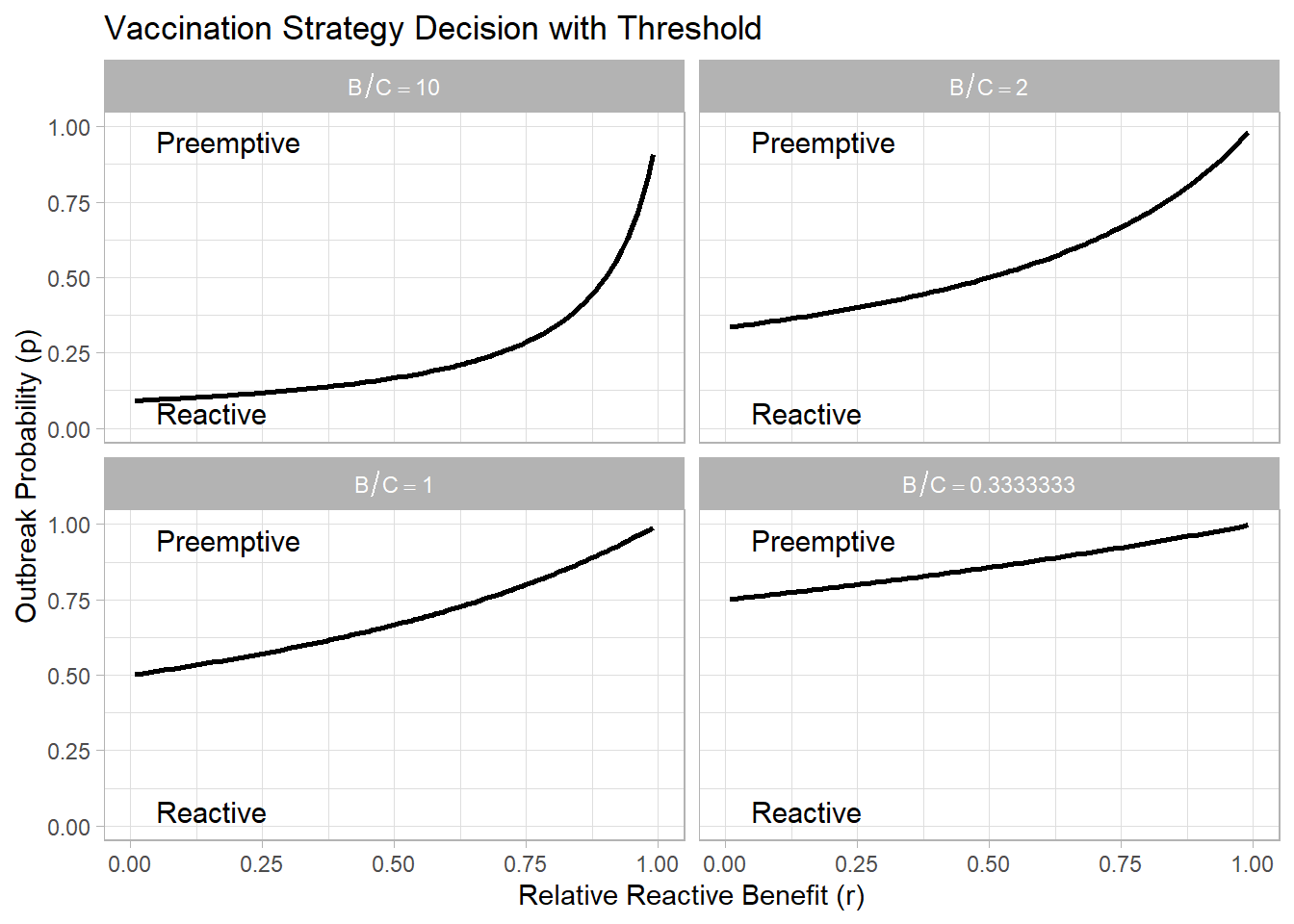
4.2.1.3 \(p_{\mathrm{crit}}^{(n)}\) in case of multi-population of equal-risk for \(f = 0.5\):

Phase diagram of reactive and pre-emptive strategies across \(r\) and \(R\). Lines represent \(p_{\mathrm{crit}}^{(n)}\) for different values of \(R\).

Code

r_vals  <- seq(0, 1, by = 0.005)
R_vals  <- c(0.1, 1, 10)
f_val   <- 0.5

df_multi <- expand.grid(r = r_vals, R = R_vals) |>
  dplyr::rowwise() |>
  dplyr::mutate(p_star = p_star_multi(R = R, r = r, f = f_val, nu = 1)) |>
  dplyr::ungroup()

ggplot(df_multi, aes(x = r, y = p_star, color = factor(R))) +
  geom_line(linewidth = 1) +
  geom_abline(slope = 1, intercept = 0,
              linetype = "dotted",
              linewidth = 1, color = "firebrick") +
  geom_abline(slope = 0, intercept = f_val,
              linetype = "dotted",
              linewidth = 1, color = "steelblue") +
  scale_y_continuous(limits = c(0, 1)) +
  labs(
    x = expression(italic(r)),
    # y = expression(italic(p)[crit]^(italic(n))),
    y = expression("outbreak probability"~italic(p)),  
    color = expression(italic(R))
  ) +
  theme_light() +
  theme(legend.position = "top") +
  annotate("text", size = 4,
           x = 0, y = 1, hjust = 0, vjust = 1,
           label = "Pre-emptive\nfavored") +
  annotate("text", size = 4,
           x = 1, y = 0, hjust = 1, vjust = 0,
           label = "Reactive\nfavored")+
  annotate("text", size = 4,
           x = 1, y = f_val, hjust = 1, vjust = -0.3,
           label = expression(italic(f)))

4.2.1.4 3D surface of \(p_{\mathrm{crit}}^{(n)}\) across \(R\) and \(r\)

Code

f_val <- 0.3

r_vals <- seq(0, 1, length.out = 100)
R_vals <- 10 ^ seq(-2, 2, length.out = 100)

p_mat_n <- outer(
  R_vals, r_vals,
  Vectorize(function(R, r) p_star_multi(R = R, r = r, f = f_val, nu = 1))
)

p_mat_n_t <- t(p_mat_n)

R_pre  <- 10
r_pre  <- 0.2
p_pre_star <- p_star_multi(R = R_pre, r = r_pre, f = f_val, nu = 1)
p_pre  <- min(1, p_pre_star + 0.6)

R_reac <- 10
r_reac <- 0.8
p_reac_star <- p_star_multi(R = R_reac, r = r_reac, f = f_val, nu = 1)
p_reac <- 0.4

df_labels_n <- data.frame(
  R   = c(R_pre,  R_reac),
  r   = c(r_pre,  r_reac),
  p   = c(p_pre,  p_reac),
  lab = c("pre-emptive", "reactive")
)

p_equal_f_mat <- 
  matrix(f_val, nrow = length(r_vals), ncol = length(R_vals))

camera <- list(
  eye = list(x = 0.1, y = 0.08, z = 0.1)
)

titlefontsize <- 34
tickfontsize <- 17

fig_pstar_multi <-
  plot_ly() %>%
  add_surface(
    x = R_vals,
    y = r_vals,
    z = p_mat_n_t,
    colorscale = "Viridis",
    showscale = TRUE,
    colorbar = list(
      title = list(
        text = "<i>p</i><sub>crit</sub><sup>(<i>n</i>)</sup>",
        font = list(size = titlefontsize)
      )
    )
  ) %>%
  # add_trace(
  #   data = df_labels_n,
  #   x = ~R,
  #   y = ~r,
  #   z = ~p,
  #   type = "scatter3d",
  #   mode = "text",
  #   text = ~lab,
  #   textposition = "middle center",
  #   textfont = list(size = titlefontsize, color = "black"),
  #   showlegend = FALSE
  # ) %>%
  add_surface(
    x = R_vals,
    y = r_vals,
    z = p_equal_f_mat,
    opacity = 0.5,
    showscale = FALSE,
    colorscale = list(c(0, "grey50"), c(1, "grey50")),
    name = "p=f"
  ) %>%
  # add_trace(
  #   x = 100,
  #   y = 1,
  #   z = f_val,
  #   type = "scatter3d",
  #   mode = "text",
  #   text = "<i>p</i> = <i>f</i>",
  #   textfont = list(size = titlefontsize, color = "black"),
  #   showlegend = FALSE
  # ) %>% 
  layout(
    scene = list(
      camera = camera,
      yaxis = list(
        title = "<i>r</i>",
        titlefont = list(size = titlefontsize),
        tickfont = list(size = tickfontsize)),
      xaxis = list(
        title = "<i>R</i>",
        type  = "log",
        tickvals = c(0.01, 0.1, 1, 10, 100),
        ticktext = c("0.01", "0.1", "1", "10", "100"),
        titlefont = list(size = titlefontsize),
        tickfont = list(size = tickfontsize)
      ),
      zaxis = list(
        title = "<i>p</i>", 
        titlefont = list(size = titlefontsize),
        tickfont = list(size = tickfontsize))
    )
  )

fig_pstar_multi

4.2.1.5 Heatmap

\(f=0.3\)

Code

# Parameters
f_val <- 0.3      # capacity fraction
p_val <- 0.6      # mean outbreak probability (not directly used here)

r_vals <- seq(0, 1, length.out = 200)
R_vals <- 10 ^ seq(-2, 2, length.out = 200)

# --- 1. Heatmap data: p_crit^(n) across (R, r) ---
df_heatmap_n <- expand.grid(R = R_vals, r = r_vals) %>%
  mutate(
    p_crit_n = mapply(
      function(R_single, r_single) {
        p_star_multi(R = R_single, r = r_single, f = f_val, nu = 1)
      },
      R, r
    )
  )

# --- 2. Multiple boundary curves for p_crit^(n) ---
p_levels <- seq(0.2, 0.8, by = 0.3)

df_boundary_n <- lapply(p_levels, function(p_target) {
  tmp <- lapply(R_vals, function(RR) {
    f_root <- function(r) p_star_multi(R = RR, r = r, f = f_val, nu = 1) - p_target
    
    sol <- tryCatch(
      uniroot(f_root, interval = c(0, 1)),
      error = function(e) NULL
    )
    
    if (is.null(sol)) return(NULL)
    
    data.frame(
      R        = RR,
      r        = sol$root,
      p_target = p_target
    )
  }) %>% bind_rows()
  
  tmp
}) %>% bind_rows()

# --- 3. Midpoints along each boundary curve for annotation ---
df_boundary_labels <- df_boundary_n %>%
  group_by(p_target) %>%
  slice(round(n() / 2)) %>%
  ungroup() %>%
  mutate(
    label = sprintf("p[crit]^{(n)}==%.1f", p_target)
  )

# --- 4. Region labels (optional) ---
R_pre  <- 12
r_pre  <- 0.15
R_reac <- 12
r_reac <- 0.85

df_labels_n <- data.frame(
  R   = c(R_pre,        R_reac),
  r   = c(r_pre,        r_reac),
  lab = c("pre-emptive favored", "reactive favored")
)

# --- 5. Heatmap with multiple boundary lines (all same style) ---
ggplot(df_heatmap_n, aes(x = R, y = r)) +
  # Heatmap
  geom_raster(aes(fill = p_crit_n)) +
  
  # Boundary curves (same color, no legend)
  geom_line(
    data = df_boundary_n,
    aes(x = R, y = r, group = p_target),
    color = "firebrick",
    linewidth = 0.8
  ) +
  
  # Line labels
  geom_text(
    data  = df_boundary_labels,
    aes(x = R, y = r, label = label),
    color = "firebrick",
    size  = 3.5,
    vjust = -0.3,
    parse = TRUE
  ) +
  
  # Region labels
  geom_text(
    data = df_labels_n,
    aes(label = lab),
    color = "white",
    size = 4
  ) +
  
  # Axes
  scale_x_log10(
    breaks = c(0.01, 0.1, 1, 10, 100),
    labels = c("0.01", "0.1", "1", "10", "100"),
    expand = c(0, 0)
  ) +
  scale_y_continuous(expand = c(0, 0)) +
  
  # Colorbar
  scale_fill_viridis_c(
    option = "viridis",
    name = expression(italic(p)[crit]^{(n)})
  ) +
  
  # Axis labels
  labs(
    x = expression("Cost ratio " * italic(R) == italic(C)[I] / italic(C)[V]),
    y = expression("Reactive effectiveness  " * italic(r))
  ) +
  
  theme_minimal() +
  theme(
    panel.grid       = element_blank(),
    axis.title       = element_text(size = 14),
    axis.text        = element_text(size = 12),
    legend.title     = element_text(size = 14),
    legend.text      = element_text(size = 12),
    legend.key.height = unit(1.5, "cm")
  )

4.2.2 Critical outbreak probability \(p_{\mathrm{crit}}^{(n)}\)

Because \(c_{\mathrm{react}}^{(n)}\) is piecewise, \(p_{\mathrm{crit}}^{(n)}\) also has a piecewise form.

4.2.2.1 Case 1: capacity scarce or just sufficient (\(f \le p\))

Here the equality occurs in the reactive-limited regime, so we set \[ c_{\mathrm{pre}}^{(n)} = f + (1-f\nu)pR, \qquad c_{\mathrm{react}}^{(n)} = f + (p - fr)R. \]

Setting them equal and simplifying: \[ (1-f\nu)pR = (p-fr)R \implies p - f\nu p = p - fr \implies f\nu p = fr \implies p = \frac{r}{\nu}. \] Thus, \[ p_{\mathrm{crit}}^{(n)} = \frac{r}{\nu}. \] In this regime, the critical probability is independent of \(R\) but depends on the pre-emptive effectiveness \(\nu\) and the reactive effectiveness \(r\). This regime applies when \(p_{\mathrm{crit}}^{(n)} \ge f \iff r/\nu \ge f\).

4.2.2.2 Case 2: capacity abundant (\(f \ge p\))

Here the equality occurs in the reactive-rich regime, so we set \[ c_{\mathrm{pre}}^{(n)} = f + (1-f\nu)pR, \qquad c_{\mathrm{react}}^{(n)} = p\bigl[1 + (1-r)R\bigr]. \]

Equating and solving for \(p\): \[ f + pR - f\nu pR = p + pR - prR \\ f = p[1 + R(1 - r) - R(1 - f\nu)] \\ f = p[1 + R(f\nu - r)] \] So, \[ p_{\mathrm{crit}}^{(n)} = \frac{f}{1 + R(f\nu - r)}. \]

Consistency with the reactive-rich regime requires \(p_{\mathrm{crit}}^{(n)} \le f\), which holds whenever \(1 + R(f\nu - r) \ge 1 \iff R(f\nu - r) \ge 0 \iff f\nu \ge r\).

4.2.3 Summary

Putting the two regimes together: \[ p_{\mathrm{crit}}^{(n)}(f,r,R) = \begin{cases} \dfrac{r}{\nu}, & f \le \dfrac{r}{\nu},\\[8pt] \dfrac{f}{1 + R(f\nu - r)}, & f > \dfrac{r}{\nu}. \end{cases} \]

Interpretation:

If \(f\nu \le r\) (or \(f \le r/\nu\)), the critical outbreak probability is simply \(r/\nu\).
If \(f\nu > r\), the critical probability depends on the outbreak–to–vaccination cost ratio, \(R\):
- larger \(R\) (more costly outbreaks) \(\Rightarrow\) smaller \(p_{\mathrm{crit}}^{(n)}\),
- larger \(f\nu\) (more effective capacity) \(\Rightarrow\) larger \(p_{\mathrm{crit}}^{(n)}\), for fixed \(R\) and \(r\).

4.3 Multiple populations with equal risk and a mixed strategy

We extend the multi-population model by allowing a fraction \(0 < \alpha \leq 1\) of the vaccines \(f\) (expressed as a fraction of the population) to be used pre-emptively, while the remaining \((1 - \alpha) f\) are used reactively.

4.3.1 Strategy parameterization

Let \(f_{\mathrm{pre}}\) be the fraction vaccinated pre-emptively and \(f_{\mathrm{react}}\) the fraction reserved for reactive use.

Parameterize by a mixing weight \(\alpha \in [0,1]\):

\(f_{\mathrm{pre}} = \alpha f\)
\(f_{\mathrm{react}} = (1-\alpha)f\)
\(f_{\mathrm{pre}} + f_{\mathrm{react}} = f\)

Thus \(\alpha=1\) is pure pre-emptive and \(\alpha=0\) is pure reactive.

4.3.2 Cost model

4.3.2.1 Pre-emptive component

A fraction \(f_{\mathrm{pre}}=\alpha f\) is vaccinated regardless of whether an outbreak occurs: \[ C_{\mathrm{pre}}^{(n)} = \alpha f\, [C_{\mathrm{V}} + p(1-\nu) C_{\mathrm{I}}], \qquad c_{\mathrm{pre}}^{(n)} = \alpha f [1 + p(1-\nu)R]. \]

4.3.2.2 Reactive component and the two regimes

Among the non-pre-emptively vaccinated fraction \((1-\alpha f)\), the expected outbreak fraction is \(p(1-\alpha f)\), while reactive capacity is \((1-\alpha)f\). Two regimes arise:

Reactive-rich (enough reactive campaigns to cover all outbreaks among the non-pre-emptive group): \[ (1-\alpha)f \;\ge\; p(1-\alpha f). \]
Reactive-limited (not enough reactive campaigns): \[ (1-\alpha)f \;<\; p(1-\alpha f). \]

4.3.2.2.1 Regime A: reactive-rich

Every outbreak among the non-pre-emptive group receives a reactive campaign. For any non-pre-emptive population, the expected cost is

outbreak w.p. \(p\): \(C_V + (1-r)C_I\)
no outbreak w.p. \(1-p\): \(0\)

Hence \[ C_{\mathrm{react}}^{(n)}(\alpha) = (1-\alpha f)\,p\left(C_V + (1-r)C_I\right), \]

and the total normalized cost is

\[ c_{\mathrm{mixed}}^{(n)}(\alpha) = \alpha f [1 + p(1-\nu)R] + (1-\alpha f)\,p\left[1 + (1-r)R\right], \qquad \text{if } (1-\alpha)f \ge p(1-\alpha f). \]

4.3.2.2.2 Regime B: reactive-limited

Only a fraction of outbreaks among the non-pre-emptive group can be reactively vaccinated. The fraction of outbreaks that receive a reactive campaign is

\[ q(\alpha) = \frac{(1-\alpha)f}{p(1-\alpha f)} \in (0,1). \]

Conditioning on an outbreak in the non-pre-emptive group: - with probability \(q(\alpha)\): pay \(C_V + (1-r)C_I\), - with probability \(1-q(\alpha)\): pay \(C_I\).

A convenient simplification yields \[ C_{\mathrm{react}}^{(n)}(\alpha) = f_{\mathrm{react}} C_V + \left[(1-f_{\mathrm{pre}})p - f_{\mathrm{react}}r\right] C_I, \]

so total normalized cost becomes \[ c_{\mathrm{mixed}}^{(n)}(\alpha) = f + R\left[p - (1-\alpha)fr - \alpha f p \nu \right], \qquad \text{if } (1-\alpha)f < p(1-\alpha f). \] Equivalently, \[ c_{\mathrm{mixed}}^{(n)}(\alpha) = f + R\left[p - fr + \alpha f(r-p\nu)\right], \qquad \text{(reactive-limited)}. \]

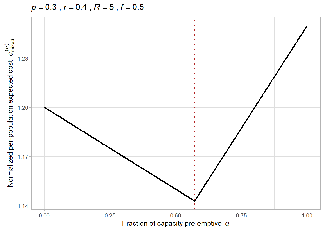
4.3.3 Geometry in \(\alpha\) and candidate optima

In both regimes, \(c_{\mathrm{mixed}}^{(n)}(\alpha)\) is affine (linear + constant) in \(\alpha\). Therefore:

within each regime, the minimizer is attained at a boundary, and
the only interior candidate is the kink where the regime switches.

Thus the global optimizer over \(\alpha \in [0,1]\) satisfies \[ \alpha^* \in \{0,\alpha_c,1\}, \] where \(\alpha_c\) is the regime-switch point.

4.3.3.1 Regime-switch point \(\alpha_c\)

Solve the boundary condition

\[ (1-\alpha)f = p(1-\alpha f). \] For \(f>p\), this yields

\[ \alpha_c = \frac{f-p}{f(1-p)} \in (0,1). \]

\((f-p)\) represents the surplus capacity available if acting purely reactively.

Now, consider the “cost” of shifting doses to pre-emptive vaccination:

Net cost of one pre-emptive dose: When you use 1 dose pre-emptively:
- You spend 1 dose from your stockpile.
- You prevent an outbreak with probability \(p\), saving \(p\) expected future reactive doses.
- The net reduction in your surplus is \(1 - p\). (This is the “waste” rate).
Maximum allowable pre-emptive doses: How many pre-emptive doses (\(D_{\mathrm{pre}}\)) can you afford? You can continue until you have consumed your entire surplus: \[ D_{\mathrm{pre}} \times (\text{Net Cost}) = \text{Surplus} \] \[ D_{\mathrm{pre}} \times (1 - p) = f - p \] \[ D_{\mathrm{pre}} = \frac{f - p}{1 - p} \]
Converting to a fraction (\(\alpha_c\)): To find the critical fraction of your total capacity (\(f\)), we divide the allowable doses by the total supply \(f\): \[ \alpha_c = \frac{D_{\mathrm{pre}}}{\text{total cpacity}} = \frac{\left( \frac{f - p}{1 - p} \right)}{f} = \frac{f - p}{f(1 - p)}. \]

Thus, the factor \(f(1-p)\) in the denominator arises from dividing the absolute surplus (\(f-p\)) by the waste rate (\(1-p\)) to get doses, and then dividing by \(f\) to get the fraction.

If \(f \le p\), then \(\alpha_c \le 0\) and the reactive-rich regime is not attainable for any \(\alpha \in [0,1]\) (reactive capacity is always limited).

4.3.4 Closed-form optimal strategy \(\alpha^*\)

Let \(\alpha^*\) denote the optimal fraction of capacity allocated to pre-emptive vaccination.

4.3.4.1 1. Scarce capacity: \(f \le p\)

Reactive capacity is always limited. From the reactive-limited cost

\[ c_{\mathrm{mixed}}^{(n)}(\alpha)=f + R\left[p-fr+\alpha f(r-p)\right], \]

the slope in \(\alpha\) is proportional to \((r-p)\), so

\[ \alpha^* = \begin{cases} 0, & r > p\nu \quad (\text{pure reactive})\\ 1, & r < p\nu \quad (\text{pure pre-emptive})\\ \text{any }\alpha \in [0,1], & r = p\nu. \end{cases} \]

4.3.4.2 2. Abundant capacity: \(f > p\)

Now \(\alpha_c \in (0,1)\) is feasible.

If \(r < p\), the reactive-limited cost decreases with \(\alpha\), so \(\alpha^*=1\) (pure pre-emptive).
If \(r > p\), compare the two corners \(\alpha=0\) (pure reactive) and \(\alpha=\alpha_c\) (largest feasible pre-emptive share while keeping the remaining group reactive-rich).

The switching critical value is

\[ R_{\mathrm{crit}} = \frac{1-p}{p(\nu-r)}. \]

Then

\[ \alpha^* = \begin{cases} 0, & r > p\nu \text{ and } R < R_{\mathrm{crit}} \quad (\text{pure reactive})\\ \alpha_c, & r > p\nu \text{ and } R \ge R_{\mathrm{crit}} \quad (\text{mixed at the kink})\\ 1, & r < p\nu \quad (\text{pure pre-emptive}). \end{cases} \]

\(\alpha_c\) is not found by minimizing a smooth function; it is the feasibility limit for staying reactive-rich among the remaining populations. It is the largest pre-emptive share such that the remaining reactive stockpile can still cover all expected outbreaks in the non-pre-emptive group.

When \(r>p\) and \(f>p\), the choice is between:

vaccinate reactively only (saving vaccines when no outbreak occurs), versus
vaccinate some pre-emptively to guarantee reactive-richness for the remainder.

\(R_{\mathrm{crit}}\) is the outbreak cost ratio at which these two options have equal expected cost; it increases as reactive effectiveness improves (as \(1-r\) shrinks).

Helper functions

Code

# Mixed strategy cost c_mix^{(n)}(alpha) = C_mix^{(n)} / C_V
cost_mix_multi <- function(alpha, p, R, r, f, nu = 1) {
  alpha <- pmax(pmin(alpha, 1), 0)

  f_pre   <- alpha * f
  f_react <- (1 - alpha) * f

  # Reactive-rich among non-pre-emptive populations
  cond_rich <- f_react >= p * (1 - f_pre)

  c_rich <- f_pre * (1 + p * (1 - nu) * R) + (1 - f_pre) * p * (1 + (1 - r) * R)
  c_lim  <- f + R * (p - f_pre * p * nu - f_react * r)

  ifelse(cond_rich, c_rich, c_lim)
}

# Numerical optimizer over a grid (useful for plotting / validation)
opt_alpha_equalrisk <- function(p, R, r, f, nu = 1, grid_len = 1001) {
  alpha_grid <- seq(0, 1, length.out = grid_len)
  costs <- cost_mix_multi(alpha = alpha_grid, p = p, R = R, r = r, f = f, nu = nu)

  idx_min <- which.min(costs)

  list(
    alpha_star = alpha_grid[idx_min],
    cost_star  = costs[idx_min],
    alpha_grid = alpha_grid,
    cost_grid  = costs
  )
}

# Closed-form alpha^* for equal-risk multi-population case
alpha_star_equalrisk <- function(p, R, r, f, nu = 1, eps = 1e-12) {
  # r can be a vector
  
  # Scarce capacity: f <= p
  if (f <= p + eps) {
    # If r > p*nu -> pure reactive (0)
    # If r < p*nu -> pure pre-emptive (1)
    return(
      ifelse(r > p * nu + eps, 0,
      ifelse(r < p * nu - eps, 1, NA_real_))
    )
  }

  # Abundant capacity: f > p
  alpha_c <- (f - p) / (f * (1 - p))

  alpha_star <- rep(NA_real_, length(r))

  # r < p*nu -> pure pre-emptive
  alpha_star[r < p * nu - eps] <- 1

  # r > p*nu -> compare alpha=0 vs alpha=alpha_c
  idx <- which(r > p * nu + eps)
  if (length(idx) > 0) {
    # R_thr = (1-p) / (p*(nu - r)) if nu > r
    # If nu <= r, slope is positive => pure reactive (alpha=0)
    
    # We set alpha_star to 0 by default for these indices
    alpha_star[idx] <- 0
    
    # Check where nu > r (slope could be negative)
    # Actually, R_thr is valid only if nu > r. 
    # If nu <= r, then 1-p + pR(r-nu) > 0 always (since 1-p>0, p>0, R>0, r>=nu).
    # So if nu <= r, pure reactive is always better. 
    
    # We only consider switching to alpha_c if nu > r AND R >= R_thr
    sub_idx <- idx[nu > r[idx] + eps] 
    
    if (length(sub_idx) > 0) {
        # Calculate R_thr for these
        R_vals_sub <- if(length(R)==1) rep(R, length(sub_idx)) else R[sub_idx]
        
        R_thr <- (1 - p) / (p * (nu - r[sub_idx]))
        
        # If R >= R_thr, switch to alpha_c
        switch_mask <- R_vals_sub >= R_thr - eps
        
        # Map sub_idx back to alpha_star
        alpha_star[sub_idx[switch_mask]] <- alpha_c
    }
  }

  alpha_star
}

4.3.4.3 \(c_{\mathrm{mixed}}^{(n)}(\alpha)\) and \(\alpha^*\)

Code

p <- 0.3
R <- 5
r <- 0.4
f <- 0.5

opt_res <- opt_alpha_equalrisk(p = p, R = R, r = r, f = f, nu = 1, grid_len = 1001)

df <- data.frame(alpha = opt_res$alpha_grid, cost = opt_res$cost_grid)
alpha_star_num  <- opt_res$alpha_star
alpha_star_anal <- alpha_star_equalrisk(p = p, R = R, r = r, f = f, nu = 1, eps = 1e-6)

ggplot(df, aes(x = alpha, y = cost)) +
  geom_line(linewidth = 1) +
  # geom_vline(xintercept = alpha_star_num, linetype = "dashed", linewidth = 0.9) +
  geom_vline(xintercept = alpha_star_anal, linetype = "dotted", 
             color = "firebrick", linewidth = 0.9) +
  labs(
    title = bquote(italic(p) == .(p) ~ "," ~ italic(r) == .(r) ~ "," ~
                   italic(R) == .(R) ~ "," ~ italic(f) == .(f)),
    x = expression("Fraction of capacity pre-emptive " ~ italic(alpha)),
    y = expression("Normalized per-population expected cost " ~ italic(c)[mixed]^{(italic(n))})
  ) +
  theme_light()

4.3.4.4 \(\alpha^*\) across \(r\)

Code

R_val <- 5
p_val <- 0.3
f_val <- 0.5

# grid

df_alpha <- data.frame(r = seq(0, 1, by = 0.001))
df_alpha$alpha_star <- alpha_star_equalrisk(
  r = df_alpha$r, R = R_val, p = p_val, f = f_val, nu = 1
)

# alpha_c

alpha_c <- ifelse(
  f_val > p_val,
  (f_val - p_val) / (f_val * (1 - p_val)),
  NA_real_
)

# r where R = R_thr(r) = (1-p)/(p(nu-r)) => nu - r = (1-p)/pR => r = nu - (1-p)/pR
nu_val <- 1
r_thr <- nu_val - (1 - p_val) / (p_val * R_val)
r_thr <- pmin(1, pmax(0, r_thr))

# --- FORCE DISCONNECTIONS (create NA gaps) ---

dr <- df_alpha$r[2] - df_alpha$r[1]     # step size (0.001 here)
gap <- 1.5 * dr                         # small gap width around thresholds

df_alpha$alpha_star[
  abs(df_alpha$r - p_val)  <= gap |
    abs(df_alpha$r - r_thr)  <= gap
] <- NA_real_

ggplot(df_alpha, aes(x = r, y = alpha_star)) +
  geom_line(linewidth = 1) +
  geom_hline(yintercept = 0, linetype = "dotted") +
  geom_hline(yintercept = 1, linetype = "dotted") +
  # p = r line + label
  geom_vline(xintercept = p_val, linetype = "dashed") +
  annotate(
    "text",
    x = p_val, y = 0.98,
    label = "italic(p)==italic(r)/nu",
    parse = TRUE,
    hjust = -0.05, vjust = 1
  ) +
  
  # R = R_crit line + label (at r = r_thr for fixed R)
  geom_vline(xintercept = r_thr, linetype = "dotted", linewidth = 1) +
  annotate(
    "text",
    x = r_thr, y = 0.90,
    label = "italic(R)==italic(R)[crit]",
    parse = TRUE,
    hjust = -0.05, vjust = 1
  ) +
  
  annotate(
    "text",
    x = max(0.02, r_thr * 0.8), y = 0.62,
    label = "italic(R) > italic(R)[crit]",
    parse = TRUE,
    hjust = 0
  ) +
  geom_hline(yintercept = alpha_c, linetype = "dashed") +
  coord_cartesian(ylim = c(0, 1)) +
  labs(
    x = expression("Reactive effectiveness " ~ italic(r)),
    y = expression("Optimal pre-emptive fraction " ~ italic(alpha)^"*"),
    title = bquote(italic(p) == .(p_val) ~ "," ~ italic(R) == .(R_val) ~ "," ~ italic(f) == .(f_val))
  ) +
  theme_light()

1 Background

2 Key Existing Studies

3 Economic costs of outbreaks and vaccination campaign

3.1 Cost of an outbreak

3.2 Cost of a cholera vaccination program

4 Scenarios

4.1 One Population

4.1.1 Pre-emptive strategy

4.1.2 Reactive strategy

4.1.3 Normalized Per-Population Expected Costs

4.1.3.1 Pre-emptive:

4.1.3.2 Reactive:

4.1.4 Critical Outbreak Probability \(p_{\mathrm{crit}}^{(1)}\)

4.1.4.1 Normalized per-population costs across \(p\) for varying \(\nu - r\).

4.1.4.1.1 Functions

4.1.4.2 Phase diagram of \(p\) vs \(r\) for \(R=1\).

4.1.4.3 \(p_{\mathrm{crit}}^{(1)}\) as a function of \(R\) for \(r=0.5\).

4.1.4.4 Heatmap of \(p_{\mathrm{crit}}^{(1)}\) across \(r\) and \(R\)

4.1.5 Key Insight

4.2 Multiple populations with equal risk and limited vaccination capacity

4.2.1 Visualization

4.2.1.1 Functions

4.2.1.2 \(c_{\mathrm{pre}}^{(n)}\) and \(c_{\mathrm{react}}^{(n)}\)

4.2.1.2.1 Low cost ratio (\(R = 1\))

4.2.1.2.2 High cost ratio (\(R = 6\))

4.2.1.3 \(p_{\mathrm{crit}}^{(n)}\) in case of multi-population of equal-risk for \(f = 0.5\):

4.2.1.4 3D surface of \(p_{\mathrm{crit}}^{(n)}\) across \(R\) and \(r\)

4.2.1.5 Heatmap

4.2.2 Critical outbreak probability \(p_{\mathrm{crit}}^{(n)}\)

4.2.2.1 Case 1: capacity scarce or just sufficient (\(f \le p\))

4.2.2.2 Case 2: capacity abundant (\(f \ge p\))

4.2.3 Summary

4.3 Multiple populations with equal risk and a mixed strategy

4.3.1 Strategy parameterization

4.3.2 Cost model

4.3.2.1 Pre-emptive component

4.3.2.2 Reactive component and the two regimes

4.3.2.2.1 Regime A: reactive-rich

4.3.2.2.2 Regime B: reactive-limited

4.3.3 Geometry in \(\alpha\) and candidate optima

4.3.3.1 Regime-switch point \(\alpha_c\)

4.3.4 Closed-form optimal strategy \(\alpha^*\)

4.3.4.1 1. Scarce capacity: \(f \le p\)

4.3.4.2 2. Abundant capacity: \(f > p\)

4.3.4.3 \(c_{\mathrm{mixed}}^{(n)}(\alpha)\) and \(\alpha^*\)

4.3.4.4 \(\alpha^*\) across \(r\)

4.4 References