Physics-Informed Neural Networks for Epidemic Modeling

Fitting SIR dynamics and recovering transmission parameters with a physics-constrained network

1 From neural ODEs to PINNs: a brief history

The idea of using neural networks to solve differential equations is older than deep learning itself. Lagaris et al. (1) showed in 1998 that a simple feedforward network, trained to minimise the residual of an ODE or PDE, could approximate analytical solutions across a spatial or temporal domain. The key insight was that automatic differentiation makes the ODE residual a differentiable loss term, enabling gradient-based training without a numerical solver.

Raissi et al. (2) named and systematised this idea as Physics-Informed Neural Networks: embedding known governing equations — ODEs, PDEs, integral equations, or any other physical constraints — directly into the loss function. Their framework covered:

• Forward problems — given the parameters and initial conditions, solve for the solution trajectory; the PINN provides a mesh-free, differentiable approximation to the ODE/PDE solution.
• Inverse problems — given noisy observations of the solution, infer the unknown parameters; \(\beta\) and \(\gamma\) are simply treated as additional learnable parameters of the model alongside the network weights.

The paper demonstrated PINNs on canonical fluid-dynamics problems (Navier–Stokes, Burgers equation) and attracted follow-on interest in physics, engineering, and biology.

2 PINNs in epidemiology and infectious diseases

In a COVID-19 application, Linka et al. (3) embedded a SEIR model inside a PINN to estimate time-varying transmission rates from reported case counts across European countries. The physics constraint stabilised parameter recovery even when surveillance data were noisy and incomplete.

Kharazmi et al. (4) demonstrated the approach more rigorously on integer- and fractional-order compartmental models, showing that PINNs can reliably identify structural and parametric features of epidemic models from sparse time-series. Their framework, developed within the Karniadakis group that produced the original PINN paper, introduced careful treatment of identifiability — a critical concern when inferring multiple epidemic parameters simultaneously.

A recurring theme across these studies is that the physics residual acts as a regulariser: by penalising solutions that violate the physics equations, the network is prevented from overfitting the noisy observations, and the inferred parameters reflect the underlying epidemic dynamics rather than noise artefacts.

More recent work has extended PINNs to:

• Multi-wave dynamics — multi-phase PINNs that switch physics regimes across intervention periods, capturing policy-driven changes in \(\beta\) (5).
• Fractional-order models — incorporating memory effects through fractional derivatives to better match empirical epidemic decay curves (4).
• Uncertainty quantification — Bayesian PINN extensions that propagate uncertainty in parameters through to forecast intervals (6).
• Wastewater surveillance — fitting PINNs to environmental sentinel data is a natural next step, though published applications remain limited.

In the following, I use a simple SIR model to demonstrate how PINNs work.

Tip

What you need

pip install torch scipy matplotlib numpy

Code tested with: torch 2.11, scipy 1.17, Python 3.11.

---

3 The SIR model

The SIR model partitions a closed population of size \(N\) into:

• \(S(t)\): Susceptible — not yet infected
• \(I(t)\): Infectious — currently infected and able to transmit
• \(R(t)\): Recovered — immune (or deceased)

The dynamics are:

\[ \frac{dS}{dt} = -\frac{\beta S I}{N}, \qquad \frac{dI}{dt} = \frac{\beta S I}{N} - \gamma I, \qquad \frac{dR}{dt} = \gamma I \]

Parameter	Meaning	Units
\(\beta\)	transmission rate	contacts / day × probability / contact
\(\gamma\)	recovery rate	1 / day
\(R_0 = \beta/\gamma\)	basic reproduction number	dimensionless

Throughout this post we use \(\beta = 0.3\), \(\gamma = 0.1\) (\(R_0 = 3\)) as the data-generating truth.

---

4 Simulate ground truth and noisy observations

import numpy as np
import torch
import torch.nn as nn
from scipy.integrate import odeint as scipy_odeint
import matplotlib.pyplot as plt

# Reproducibility
torch.manual_seed(42)
np.random.seed(42)

plt.rcParams.update({
    "figure.dpi": 130,
    "axes.spines.top": False,
    "axes.spines.right": False,
    "axes.grid": True,
    "grid.alpha": 0.3,
    "font.size": 11,
})

C_S, C_I, C_R   = "#2196F3", "#F44336", "#4CAF50"
C_OBS, C_PINN   = "black", "#9C27B0"

# --- Ground truth parameters ---
N          = 1_000
beta_true  = 0.3
gamma_true = 0.1
T_max      = 60.0

y0 = np.array([990.0, 10.0, 0.0])

def sir_rhs(y, t, beta, gamma, N):
    S, I, R = y
    return [-beta*S*I/N, beta*S*I/N - gamma*I, gamma*I]

n_grid = 100
t_grid = np.linspace(0, T_max, n_grid)
sol    = scipy_odeint(sir_rhs, y0, t_grid, args=(beta_true, gamma_true, N))
S_true, I_true, R_true = sol.T

print(f"R₀ = {beta_true/gamma_true:.1f}")
print(f"Peak infections: {I_true.max():.0f} on day {t_grid[I_true.argmax()]:.1f}")
print(f"Final susceptibles: {S_true[-1]:.0f}")

# --- Sparse, noisy observations of I(t) only ---
n_obs   = 30
obs_idx = np.sort(np.random.choice(np.arange(1, n_grid), n_obs, replace=False))
t_obs   = t_grid[obs_idx]
I_obs   = np.clip(I_true[obs_idx] + np.random.normal(0, 20.0, n_obs), 0, N)

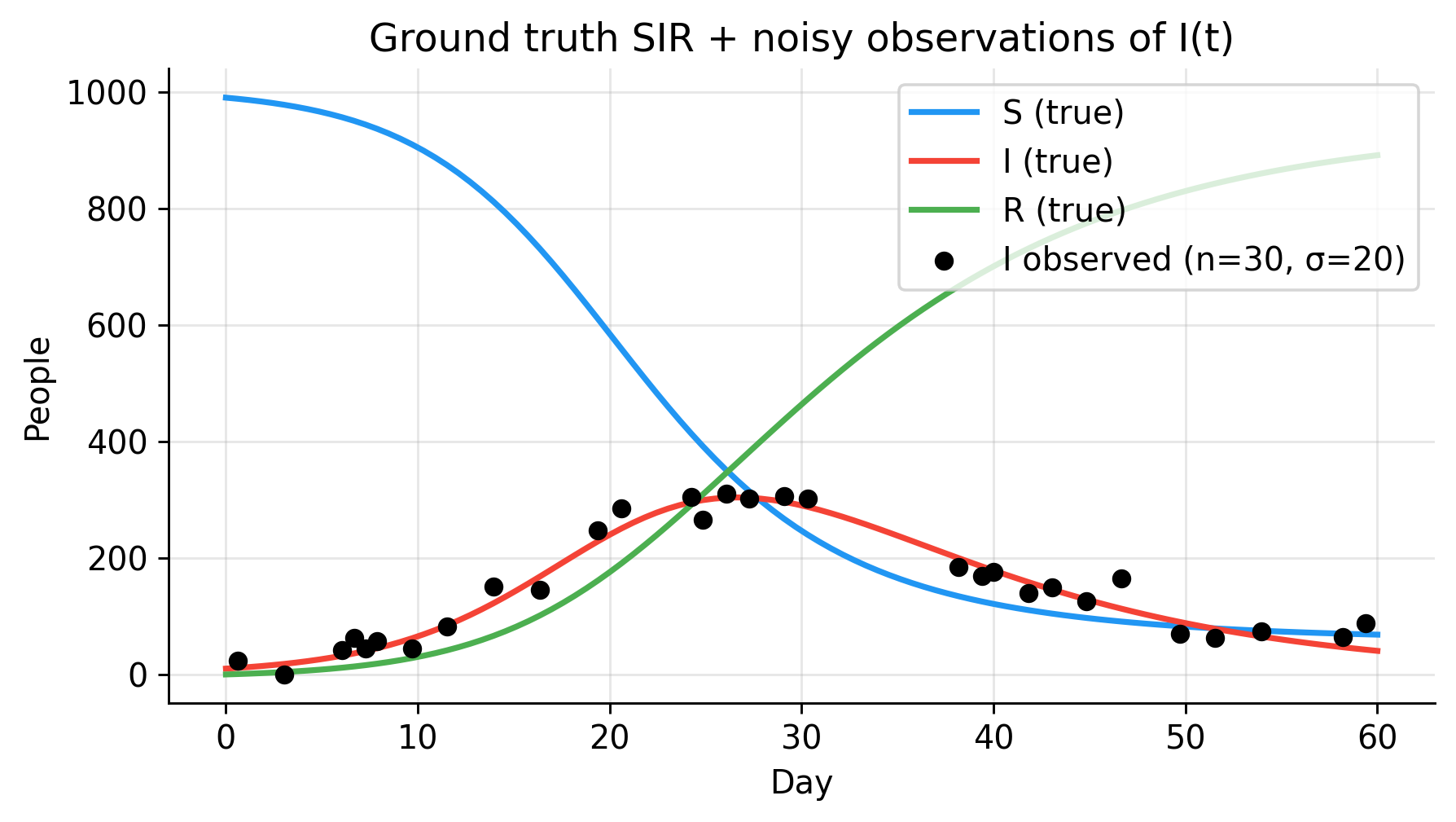
fig, ax = plt.subplots(figsize=(7, 4))
ax.plot(t_grid, S_true, color=C_S, lw=2, label="S (true)")
ax.plot(t_grid, I_true, color=C_I, lw=2, label="I (true)")
ax.plot(t_grid, R_true, color=C_R, lw=2, label="R (true)")
ax.scatter(t_obs, I_obs, color=C_OBS, s=30, zorder=5,
           label=f"I observed (n={n_obs}, σ=20)")
ax.set(xlabel="Day", ylabel="People",
       title="Ground truth SIR + noisy observations of I(t)")
ax.legend(loc="upper right")
plt.tight_layout()
plt.show()

R₀ = 3.0
Peak infections: 304 on day 26.7
Final susceptibles: 68

Only the black dots are available for training. The full \(S\), \(I\), \(R\) trajectories are hidden from the model.

---

5 Physics-Informed Neural Network

5.1 Architecture

A PINN maps scaled time \(t_s \in [0,1]\) directly to the three compartment proportions \((S/N, I/N, R/N)\):

\[ (S(t),\, I(t),\, R(t)) / N \;=\; \text{NN}_\theta(t/T_{\max}) \]

Two scalar scalars — \(\log\beta_s\) and \(\log\gamma_s\) (log of the scaled-time parameters) — are additional learnable parameters of the model (i.e., in addition to the network weights and biases). Physical rates are recovered as \(\beta = \beta_s / T_{\max}\), \(\gamma = \gamma_s / T_{\max}\).

class PINN(nn.Module):
    """
    Physics-Informed Neural Network for the SIR model.

    Input  : scaled time t_s ∈ [0, 1]   — shape (batch,)
    Output : (S, I, R) / N proportions  — shape (batch, 3)

    Learnable epidemic parameters
    -----------------------------
    log_beta_s, log_gamma_s : log of β and γ in scaled-time units.
        Physical rates: β = exp(log_beta_s) / T_max
    """
    def __init__(self, hidden: int = 64, depth: int = 4):
        super().__init__()
        layers = [nn.Linear(1, hidden), nn.Tanh()]
        for _ in range(depth - 1):
            layers += [nn.Linear(hidden, hidden), nn.Tanh()]
        layers += [nn.Linear(hidden, 3), nn.Sigmoid()]
        self.net = nn.Sequential(*layers)

        # Initialise near plausible values
        # True scaled params: β_s = 0.3 × 60 = 18, γ_s = 0.1 × 60 = 6
        self.log_beta_s  = nn.Parameter(torch.tensor(np.log(10.0)))
        self.log_gamma_s = nn.Parameter(torch.tensor(np.log( 3.0)))

    @property
    def beta_s(self):    return torch.exp(self.log_beta_s)
    @property
    def gamma_s(self):   return torch.exp(self.log_gamma_s)
    @property
    def beta_phys(self): return self.beta_s  / T_max
    @property
    def gamma_phys(self):return self.gamma_s / T_max
    @property
    def R0_est(self):    return self.beta_s  / self.gamma_s   # scale-invariant

    def forward(self, t_s):
        return self.net(t_s.view(-1, 1))   # (batch, 3)

5.2 Loss functions

Training minimises a composite loss:

\[ \mathcal{L} = \underbrace{\mathcal{L}_\text{data}}_{\text{fit I observations}} + \lambda_\phi \underbrace{\mathcal{L}_\text{physics}}_{\text{SIR residuals via autograd}} + \lambda_0 \underbrace{\mathcal{L}_\text{IC}}_{\text{initial conditions}} \]

The data loss \(\mathcal{L}_\text{data}\) is the MSE between predicted \(I(t)\) at the 30 observation times and the noisy counts — the only observed signal.

The physics loss \(\mathcal{L}_\text{physics}\) uses automatic differentiation to evaluate the SIR residuals at 200 collocation points spread across \([0, T_{\max}]\). Working in scaled time \(t_s = t/T_{\max}\), the SIR ODEs become:

\[ \frac{dS}{dt_s} = -\beta_s S I, \qquad \frac{dI}{dt_s} = \beta_s S I - \gamma_s I, \qquad \frac{dR}{dt_s} = \gamma_s I \]

The initial-condition loss \(\mathcal{L}_\text{IC}\) pins the network to the known state at \(t = 0\), preventing the network from drifting to arbitrary solutions.

def data_loss(model, t_obs_s, I_obs_s):
    """MSE on the I compartment at observed time points."""
    sir = model(t_obs_s)
    return ((sir[:, 1] - I_obs_s) ** 2).mean()


def physics_loss(model, t_col_base):
    """
    SIR residuals at collocation points via automatic differentiation.
    Operates entirely in scaled time — no solver required.
    """
    t = t_col_base.clone().requires_grad_(True)
    sir = model(t)
    S, I, R = sir[:, 0], sir[:, 1], sir[:, 2]

    ones = torch.ones(len(t))
    dS = torch.autograd.grad(S, t, grad_outputs=ones, create_graph=True)[0]
    dI = torch.autograd.grad(I, t, grad_outputs=ones, create_graph=True)[0]
    dR = torch.autograd.grad(R, t, grad_outputs=ones, create_graph=True)[0]

    b, g = model.beta_s, model.gamma_s
    res_S = dS + b * S * I
    res_I = dI - b * S * I + g * I
    res_R = dR - g * I

    return (res_S**2 + res_I**2 + res_R**2).mean()


def ic_loss(model, y0_s):
    """Match (S0, I0, R0)/N at t = 0."""
    sir0 = model(torch.tensor([0.0]))[0]
    return ((sir0 - y0_s) ** 2).mean()

Note

Why collocation points?

The physics loss is evaluated on a dense grid (200 points) that is separate from the sparse observation times (30 points). These collocation points are chosen to cover the full integration window, so the SIR residual is penalised everywhere — not just where data exist. This is the mechanism by which physics knowledge extrapolates the data signal.

5.3 Training

# Tensors — everything scaled to [0, 1]
t_obs_s = torch.tensor(t_obs / T_max, dtype=torch.float32)
I_obs_s = torch.tensor(I_obs / N,     dtype=torch.float32)
y0_s    = torch.tensor(y0   / N,      dtype=torch.float32)
t_col   = torch.linspace(0, 1, 200)

# Loss weights
lam_phys = 0.1
lam_ic   = 5

pinn        = PINN(hidden=64, depth=4)
opt         = torch.optim.Adam(pinn.parameters(), lr=1e-3)
sched       = torch.optim.lr_scheduler.StepLR(opt, step_size=2000, gamma=0.5)

losses     = []
beta_hist  = []
gamma_hist = []

for epoch in range(6_000):
    opt.zero_grad()

    L_data  = data_loss(pinn, t_obs_s, I_obs_s)
    L_phys  = physics_loss(pinn, t_col)
    L_ic    = ic_loss(pinn, y0_s)
    loss    = L_data + lam_phys * L_phys + lam_ic * L_ic

    loss.backward()
    nn.utils.clip_grad_norm_(pinn.parameters(), max_norm=1.0)
    opt.step()
    sched.step()

    losses.append(loss.item())
    beta_hist.append(pinn.beta_phys.item())
    gamma_hist.append(pinn.gamma_phys.item())

print(f"True:      β = {beta_true:.3f}, γ = {gamma_true:.3f}, R₀ = {beta_true/gamma_true:.2f}")
print(f"PINN est.: β = {pinn.beta_phys.item():.3f}, "
      f"γ = {pinn.gamma_phys.item():.3f}, "
      f"R₀ = {pinn.R0_est.item():.2f}")

True:      β = 0.300, γ = 0.100, R₀ = 3.00
PINN est.: β = 0.295, γ = 0.098, R₀ = 3.01

---

6 Results

6.1 Trajectory reconstruction

t_viz_np = np.linspace(0, T_max, 300)
t_viz_s  = torch.tensor(t_viz_np / T_max, dtype=torch.float32)

with torch.no_grad():
    pred = pinn(t_viz_s).numpy() * N

sol_viz = scipy_odeint(sir_rhs, y0, t_viz_np, args=(beta_true, gamma_true, N))

fig, axes = plt.subplots(1, 2, figsize=(7, 3.5))

# Left: compartment trajectories
ax = axes[0]
for i, (label, color, true) in enumerate(
    [("S", C_S, sol_viz[:,0]), ("I", C_I, sol_viz[:,1]), ("R", C_R, sol_viz[:,2])]
):
    ax.plot(t_viz_np, true,       color=color, lw=2, ls="--", alpha=0.5,
            label=f"{label} true")
    ax.plot(t_viz_np, pred[:, i], color=color, lw=2,
            label=f"{label} PINN")
ax.scatter(t_obs, I_obs, color=C_OBS, s=25, zorder=5, label="I observed")
ax.set(xlabel="Day", ylabel="People",
       title="PINN — compartment reconstruction")
ax.legend(fontsize=8, ncol=2)

# Right: training loss
ax = axes[1]
ax.semilogy(losses, color=C_PINN, lw=1.5)
ax.set(xlabel="Epoch", ylabel="Total loss (log scale)",
       title="PINN — training curve")

plt.tight_layout()
plt.show()

The PINN fits the observed \(I(t)\) points and simultaneouly reconstructs the latent \(S(t)\) and \(R(t)\) trajectories. The physics loss ensures the predicted compartments satisfy the SIR equations everywhere, not only at the observation times.

6.2 Effect of the physics loss weight

The loss weight \(\lambda_\phi\) trades off data fidelity and physics constraint strength. Below we visualise how varying \(\lambda_\phi\) over several orders of magnitude affects the fit and the parameter estimates.

lam_values  = [0.0, 0.01, 0.1, 1.0]
lam_labels  = [f"λ={v}" for v in lam_values]
colors_lam  = ["#E91E63", "#FF9800", "#9C27B0", "#009688"]

fig, axes = plt.subplots(1, 2, figsize=(7, 3.5))

for lam, label, col in zip(lam_values, lam_labels, colors_lam):
    torch.manual_seed(42)
    m   = PINN(hidden=64, depth=4)
    opt_= torch.optim.Adam(m.parameters(), lr=1e-3)
    sch_= torch.optim.lr_scheduler.StepLR(opt_, step_size=2000, gamma=0.5)

    for _ in range(6_000):
        opt_.zero_grad()
        L = (data_loss(m, t_obs_s, I_obs_s)
             + lam * physics_loss(m, t_col)
             + lam_ic * ic_loss(m, y0_s))
        L.backward()
        nn.utils.clip_grad_norm_(m.parameters(), 1.0)
        opt_.step(); sch_.step()

    with torch.no_grad():
        p = m(t_viz_s).numpy() * N
    axes[0].plot(t_viz_np, p[:, 1], color=col, lw=1.8, label=label)
    axes[1].scatter([lam if lam > 0 else 1e-3],
                    [m.beta_phys.item()], color=col, s=80, zorder=5)
    axes[1].scatter([lam if lam > 0 else 1e-3],
                    [m.gamma_phys.item()], color=col, marker="D", s=80, zorder=5)

axes[0].plot(t_viz_np, sol_viz[:, 1], color=C_I, lw=2, ls="--",
             alpha=0.6, label="I true")
axes[0].scatter(t_obs, I_obs, color=C_OBS, s=20, zorder=5, label="Observed")
axes[0].set(xlabel="Day", ylabel="Infectious I", title="I(t) fit vs. λ_phys")
axes[0].legend(fontsize=8)

axes[1].axhline(beta_true,  color=C_I, lw=1.5, ls="--", label=f"β true={beta_true}")
axes[1].axhline(gamma_true, color=C_R, lw=1.5, ls="--", label=f"γ true={gamma_true}")
axes[1].set(xscale="log", xlabel="λ_phys", ylabel="Estimated parameter",
            title="Parameter recovery vs. λ_phys")
axes[1].legend(fontsize=8)

plt.tight_layout()
plt.show()

With \(\lambda_\phi = 0\) the network is a pure data-fitting exercise and parameter recovery collapses. Increasing \(\lambda_\phi\) pulls the estimates toward the true values; too large a weight can sacrifice data fit. In practice, \(\lambda_\phi \approx 0.1\) strikes a reasonable balance for this example.

6.3 Parameter recovery during training

fig, axes = plt.subplots(1, 2, figsize=(7, 3.5))

for ax, hist, true_val, label, color in [
    (axes[0], beta_hist,  beta_true,  "β (transmission rate)", C_I),
    (axes[1], gamma_hist, gamma_true, "γ (recovery rate)",     C_R),
]:
    ax.plot(hist, color=color, lw=1.5, label="PINN estimate")
    ax.axhline(true_val, color="black", lw=1.5, ls="--",
               label=f"True = {true_val}")
    ax.set(xlabel="Epoch", ylabel=label,
           title=f"Parameter recovery: {label}")
    ax.legend()

plt.tight_layout()
plt.show()

print(f"\nParameter recovery summary")
print(f"  β  — true: {beta_true:.3f}  |  estimated: {pinn.beta_phys.item():.3f}")
print(f"  γ  — true: {gamma_true:.3f}  |  estimated: {pinn.gamma_phys.item():.3f}")
print(f"  R₀ — true: {beta_true/gamma_true:.2f}  |  estimated: {pinn.R0_est.item():.2f}")

Parameter recovery summary
  β  — true: 0.300  |  estimated: 0.295
  γ  — true: 0.100  |  estimated: 0.098
  R₀ — true: 3.00  |  estimated: 3.01

---

7 What the PINN gives you

Property	Value
Fits \(I(t)\) observations	✓
Reconstructs \(S(t)\), \(R(t)\) without observing them	✓
Recovers \(\beta\), \(\gamma\) jointly	✓
Enforces \(S+I+R \approx N\)	✓ (via IC + physics loss)
Extrapolates beyond training window	Better than unconstrained networks
Requires an ODE solver during training	✗ (only autograd needed)
Black-box right-hand side	✗ (mechanistic residuals are explicit)

Important

The epidemiological payoff

In real outbreak settings, surveillance provides only partial, delayed, and noisy signal — exactly the scenario simulated here. The PINN framework lets you:

1. Estimate \(R_0\) from early epidemic data without knowing the final attack size.
2. Reconstruct the full population trajectory (\(S\), \(I\), \(R\)) from reported cases alone.
3. Propagate uncertainty by treating \(\beta\) and \(\gamma\) as random variables in a Bayesian PINN extension.

This is why hybrid mechanistic-AI approaches are a frontier in infectious disease forecasting.

---

8 Extensions worth exploring

More realistic compartmental structures

• Replace SIR with SEIR (add an Exposed compartment) or SEIRS (waning immunity).
• Add time-varying \(\beta(t)\) — parameterised as a second small network — to capture policy interventions or behavioural changes.
• Couple a within-host viral kinetics model to the population PINN.

Better uncertainty quantification

• Bayesian PINN: treat \(\beta\), \(\gamma\) as prior distributions and use MCMC (e.g. NUTS in NumPyro) or variational inference to obtain posterior credible intervals.
• Ensemble PINNs: train multiple networks with different random initialisations and use spread as a proxy for epistemic uncertainty.

Identifiability and multi-wave dynamics

• Not all parameters in an epidemic model are jointly identifiable from \(I(t)\) alone. Kharazmi et al. (4) provide a PINN-based identifiability analysis framework that is directly applicable to SIR extensions.
• Multi-phase PINNs split the time axis at known intervention dates and train separate physics terms for each phase — useful for fitting multi-wave outbreaks.

Real data

• Fit to weekly influenza ILI counts (CDC FluView API).
• Fit to wastewater SARS-CoV-2 concentration data (CDC NWSS), where an additional observation model links \(I(t)\) to RNA copies per litre.

Production-grade

• Replace PyTorch with JAX + Optax for cleaner functional style and XLA acceleration.
• Use the deepxde library, which wraps PINN training in a high-level API and supports arbitrary ODE/PDE geometries.

---

9 References

1.

Lagaris IE, Likas A, Fotiadis DI. Artificial neural networks for solving ordinary and partial differential equations. IEEE Transactions on Neural Networks. 1998;9(5):987–1000. doi:10.1109/72.712178

2.

Raissi M, Perdikaris P, Karniadakis GE. Physics-informed neural networks: A deep learning framework for solving forward and inverse problems involving nonlinear partial differential equations. Journal of Computational Physics. 2019;378:686–707. doi:10.1016/j.jcp.2018.10.045

3.

Linka K, Peirlinck M, Sahli Costabal F, Kuhl E. Outbreak dynamics of COVID-19 in Europe and the effect of travel restrictions. Computer Methods in Biomechanics and Biomedical Engineering. 2020;23(11):710–7. doi:10.1080/10255842.2020.1759560

4.

Kharazmi E, Cai M, Zheng X, Zhang Z, Lin G, Karniadakis GE. Identifiability and predictability of integer- and fractional-order epidemiological models using physics-informed neural networks. Nature Computational Science. 2021;1(11):744–53. doi:10.1038/s43588-021-00158-0

5.

He M, Tang B, Xiao Y, Tang S. Transmission dynamics informed neural network with application to COVID-19 infections. Computers in Biology and Medicine. 2023;165:107431. doi:10.1016/j.compbiomed.2023.107431

6.

Linka K, Schäfer A, Meng X, Zou Z, Karniadakis GE, Kuhl E. Bayesian physics informed neural networks for real-world nonlinear dynamical systems. Computer Methods in Applied Mechanics and Engineering. 2022;402:115346. doi:10.1016/j.cma.2022.115346

Python     3.12.10
torch      2.11.0+cpu
scipy      1.17.1
matplotlib 3.10.8