Transformer-Based LLM Architectures for Epidemic Time Series Forecasting

Language models tokenize text into words; time series transformers tokenize history into patches. Build a patch-attention forecaster in R that predicts four weeks of case counts from sixteen weeks of history.

1 Why epidemic forecasting needs its own transformer

The previous post showed that attention is a learned weighted average over a context window. That is the mechanism inside every LLM — GPT, Claude, Gemini — and it also underlies the best time-series forecasting models.

But applying an LLM directly to epidemic incidence data hits three structural problems:

1. Continuous vs. discrete tokens. LLMs consume discrete tokens (integers drawn from a fixed vocabulary). Case counts are continuous — a naive tokenization loses numerical structure.
2. Expensive quadratic attention. A full weekly series from 2010 to today is roughly 750 time steps. Full self-attention is \(O(n^2)\) in sequence length, which becomes expensive as history grows.
3. Distribution shift between epidemic waves. Each wave has a different scale. A model trained on a wave peaking at 2,000 cases/week struggles with a wave peaking at 200. Raw values carry absolute scale information that hurts cross-wave generalization.

Three innovations, developed between 2021 and 2024, solve each problem:

Problem	Solution	Paper
Continuous inputs	Patch embedding: segment the series into fixed-length patches; each patch becomes one “token”	PatchTST (1)
Quadratic cost	Patching also reduces sequence length by a factor of the patch length	PatchTST (1)
Distribution shift	Reversible Instance Normalization (RevIN): normalize per instance before the model, denormalize predictions afterward	Kim et al. (2)

Together they define a blueprint — patch the input, normalize it, run a transformer encoder, project to the forecast horizon — that also underlies the zero-shot foundation models TimeGPT (3) and CHRONOS (4).

This post builds that blueprint from scratch in R, using only base R, ggplot2, and dplyr.

2 The three innovations in detail

2.1 Patching: turning a time series into tokens

In an LLM, the input sentence is split into word-pieces (tokens), and the transformer attends across them. Each token carries a semantically coherent unit of meaning.

For a time series, a single time step is the equivalent of a single character — too granular to carry meaning. A patch of \(M\) consecutive time steps is the equivalent of a word: it captures a local trend, a brief acceleration, or a short plateau.

Formally, given a look-back window of \(L\) time steps, we divide it into \(P = L / M\) non-overlapping patches. The transformer then attends across \(P\) patch tokens rather than \(L\) individual steps. Reducing the sequence from \(L\) to \(P = L/M\) cuts the quadratic attention cost by a factor of \(M^2\).

2.2 RevIN: instance normalization

RevIN (2) normalises each individual input window at inference time:

\[\tilde{x}_t = \frac{x_t - \hat{\mu}}{\hat{\sigma} + \epsilon}, \quad \hat{\mu} = \frac{1}{L}\sum_{t=1}^{L} x_t, \quad \hat{\sigma} = \text{std}(x_1, \ldots, x_L)\]

The model predicts \(\tilde{y}\) in the normalized space. After prediction, the output is denormalized:

\[\hat{y}_t = \tilde{y}_t \cdot (\hat{\sigma} + \epsilon) + \hat{\mu}\]

This makes the model scale-invariant: it sees unit-variance, zero-mean inputs regardless of whether the current wave is small or large, making weights learned on one wave transfer to another.

2.3 Multi-step direct forecasting

RNNs and ARIMA produce forecasts autoregressively — one step at a time, feeding each prediction back as input. Error accumulates. A transformer encoder maps the full context to all \(H\) future steps in one shot, producing a joint forecast that is both faster and more accurate at longer horizons (5).

3 Building the patch-attention forecaster

3.1 Data: a two-wave epidemic series

set.seed(42)
n_total <- 60       # 52 weeks training + 8 weeks test
t_seq   <- 1:n_total

wave1    <- 100 * exp(-((t_seq - 18)^2) / 50)
wave2    <-  80 * exp(-((t_seq - 48)^2) / 30)
seasonal <-  15 * sin(2 * pi * t_seq / 52)
noise    <- rnorm(n_total, 0, 6)

cases <- pmax(1, round(wave1 + wave2 + seasonal + noise + 20))

n_train <- 52
n_test  <- 8
train_cases <- cases[1:n_train]
test_cases  <- cases[(n_train + 1):n_total]

cat("Training weeks:", n_train, "| Test weeks:", n_test, "\n")

Training weeks: 52 | Test weeks: 8 

cat("Case range — train:", min(train_cases), "–", max(train_cases),
    "| test:", min(test_cases), "–", max(test_cases), "\n")

Case range — train: 1 – 130 | test: 15 – 66 

3.2 Patching and RevIN helpers

L     <- 16   # look-back window (weeks)
P_len <-  4   # patch length (weeks per patch)
P     <- L / P_len   # number of patches = 4
H     <-  4   # forecast horizon (weeks ahead)

# RevIN: normalize one window, return normalized values + stats for denorm
revin_norm <- function(x) {
  mu    <- mean(x)
  sigma <- sd(x)
  list(x_norm = (x - mu) / (sigma + 1e-8), mu = mu, sigma = sigma)
}

revin_denorm <- function(x_norm, mu, sigma) {
  x_norm * (sigma + 1e-8) + mu
}

# Summarize each patch as its mean (the "embedding")
make_patch_means <- function(x_norm, patch_len) {
  n_p <- length(x_norm) / patch_len
  vapply(seq_len(n_p), function(i) {
    idx <- ((i - 1) * patch_len + 1):(i * patch_len)
    mean(x_norm[idx])
  }, numeric(1))
}

3.3 Building the training dataset

Each training sample is a (patches, targets) pair. The patches encode the normalized look-back window; the targets are the next \(H\) steps in the same normalized space.

n_samples <- n_train - L - H + 1   # = 33 training examples

X_patches  <- matrix(NA_real_, n_samples, P)
y_targets  <- matrix(NA_real_, n_samples, H)
norm_stats  <- vector("list", n_samples)   # store mu/sigma for each window

for (i in seq_len(n_samples)) {
  window    <- train_cases[i:(i + L - 1)]
  rv        <- revin_norm(window)
  norm_stats[[i]] <- rv
  X_patches[i, ] <- make_patch_means(rv$x_norm, P_len)
  future         <- train_cases[(i + L):(i + L + H - 1)]
  y_targets[i, ] <- (future - rv$mu) / (rv$sigma + 1e-8)
}

cat("Training samples:", n_samples,
    "| Patches per sample:", P,
    "| Forecast steps:", H, "\n")

Training samples: 33 | Patches per sample: 4 | Forecast steps: 4 

3.4 Patch-attention model

The model has three parameter groups:

• \(\boldsymbol{\alpha} \in \mathbb{R}^P\) — attention logits over patches; \(\mathbf{w} = \text{softmax}(\boldsymbol{\alpha})\)
• \(\mathbf{W} \in \mathbb{R}^{P \times H}\) — output projection from patch space to \(H\) future steps
• \(\mathbf{b} \in \mathbb{R}^H\) — bias

The forward pass for a batch of \(n\) samples is:

\[\mathbf{Z} = \mathbf{X} \odot \mathbf{w}^\top \quad (n \times P), \qquad \hat{\mathbf{Y}} = \mathbf{Z}\mathbf{W} + \mathbf{1}\mathbf{b}^\top \quad (n \times H)\]

where \(\odot\) broadcasts the patch weights \(\mathbf{w}\) across all rows of \(\mathbf{X}\). The attention weights \(\mathbf{w}\) scale the importance of each patch globally; the projection \(\mathbf{W}\) maps the reweighted patches to each future horizon.

softmax <- function(alpha) {
  e <- exp(alpha - max(alpha))
  e / sum(e)
}

# params layout: alpha[1:P], vec(W)[1:(P*H)], b[1:H]
forward <- function(params, X) {
  alpha <- params[seq_len(P)]
  W     <- matrix(params[(P + 1):(P + P * H)], nrow = P, ncol = H)
  b     <- params[(P + P * H + 1):(P + P * H + H)]
  w     <- softmax(alpha)
  Z     <- sweep(X, 2, w, "*")                              # n × P
  Z %*% W + matrix(b, nrow(X), H, byrow = TRUE)            # n × H
}

loss_fn <- function(params) {
  yhat <- forward(params, X_patches)
  mean((yhat - y_targets)^2)
}

3.5 Training with gradient descent

num_grad <- function(f, x, eps = 1e-5) {
  vapply(seq_along(x), function(j) {
    x1 <- x2 <- x
    x1[j] <- x1[j] + eps
    x2[j] <- x2[j] - eps
    (f(x1) - f(x2)) / (2 * eps)
  }, numeric(1))
}

set.seed(7)
n_params <- P + P * H + H    # 4 + 16 + 4 = 24
params <- c(rep(0, P), rnorm(P * H, 0, 0.1), rep(0, H))

lr       <- 0.05
n_iter   <- 2500
loss_log <- numeric(n_iter)

for (iter in seq_len(n_iter)) {
  g       <- num_grad(loss_fn, params)
  params  <- params - lr * g
  loss_log[iter] <- loss_fn(params)
}

w_learned <- softmax(params[seq_len(P)])
cat("Final training loss (normalized MSE):", round(loss_fn(params), 4), "\n\n")

Final training loss (normalized MSE): 0.5134 

cat("Learned patch attention weights:\n")

Learned patch attention weights:

cat(paste0("  patch ", seq_len(P), " (weeks ",
           (seq_len(P) - 1) * P_len + 1, "–",
           seq_len(P) * P_len, " of look-back): ",
           round(w_learned, 3)), sep = "\n")

  patch 1 (weeks 1–4 of look-back): 0.018
  patch 2 (weeks 5–8 of look-back): 0.008
  patch 3 (weeks 9–12 of look-back): 0.573
  patch 4 (weeks 13–16 of look-back): 0.4

The attention weights reveal which temporal segment the model finds most predictive. In an epidemic context, the most recent patch (weeks 13–16 of the look-back window) should receive the highest weight because short-term autocorrelation in case counts is strong — similar to what the single-step attention model found in the previous post, but now measured at the coarser patch scale.

3.6 Patching the time series

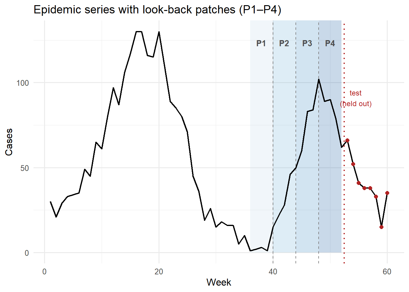
library(ggplot2)
library(dplyr)

# Build patch boundary data for the look-back window used in the test forecast
lb_start <- n_train - L + 1   # week 37
lb_end   <- n_train            # week 52

patch_df <- data.frame(
  xmin  = lb_start + (seq_len(P) - 1) * P_len - 1,
  xmax  = lb_start + seq_len(P) * P_len - 1,
  patch = factor(seq_len(P)),
  alpha_fill = seq(0.10, 0.40, length.out = P)
)

ts_df <- data.frame(week = seq_along(cases), cases = cases)

ggplot() +
  geom_rect(
    data = patch_df,
    aes(xmin = xmin, xmax = xmax, ymin = 0, ymax = Inf, fill = patch),
    alpha = 0.22, show.legend = FALSE
  ) +
  geom_vline(
    xintercept = patch_df$xmin[-1],
    linetype = "dashed", colour = "grey50", linewidth = 0.4
  ) +
  geom_line(data = ts_df, aes(x = week, y = cases),
            colour = "black", linewidth = 0.8) +
  geom_point(data = ts_df |> dplyr::filter(week > n_train),
             aes(x = week, y = cases),
             colour = "firebrick", size = 2, shape = 16) +
  scale_fill_manual(values = c("#bdd7e7", "#6baed6", "#3182bd", "#08519c")) +
  annotate("text", x = lb_start + (seq_len(P) - 0.5) * P_len - 1,
           y = max(cases) * 0.95,
           label = paste0("P", seq_len(P)),
           colour = "grey30", size = 3.5, fontface = "bold") +
  annotate("text", x = n_train + 2.5, y = max(cases) * 0.7,
           label = "test\n(held out)", colour = "firebrick", size = 3.2) +
  geom_vline(xintercept = n_train + 0.5,
             linetype = "dotted", colour = "firebrick", linewidth = 0.8) +
  labs(x = "Week", y = "Cases",
       title = "Epidemic series with look-back patches (P1–P4)") +
  theme_minimal(base_size = 12)

Figure 1: The 16-week look-back window (weeks 37–52, shaded) is divided into four patches of four weeks each. Each patch becomes one ‘token’ for the transformer encoder. The final patch (weeks 49–52, darkest shading) carries the most recent trend information and typically receives the highest attention weight.

3.7 Generating the 4-week forecast

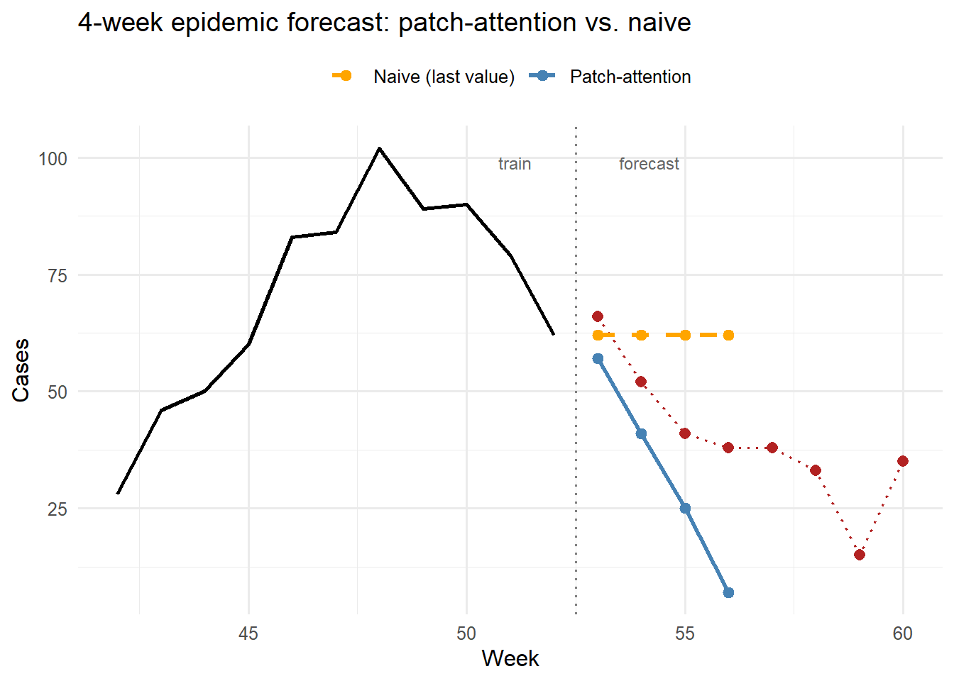
# Input window: last L=16 weeks of training data
forecast_window <- train_cases[(n_train - L + 1):n_train]
rv_test         <- revin_norm(forecast_window)
X_test          <- matrix(make_patch_means(rv_test$x_norm, P_len), nrow = 1)

# Forward pass → normalized predictions → denormalize
pred_norm  <- forward(params, X_test)
pred_cases <- pmax(0, round(revin_denorm(pred_norm[1, ], rv_test$mu, rv_test$sigma)))

# Naive baseline: repeat the last observed value
naive_pred <- rep(train_cases[n_train], H)

# Error on the first H test weeks
obs_H <- test_cases[seq_len(H)]
rmse_patch <- sqrt(mean((pred_cases - obs_H)^2))
rmse_naive <- sqrt(mean((naive_pred  - obs_H)^2))

cat("4-week forecast (patch-attention):", pred_cases, "\n")

4-week forecast (patch-attention): 57 41 25 7 

cat("4-week forecast (naive):          ", naive_pred, "\n")

4-week forecast (naive):           62 62 62 62 

cat("Observed:                         ", obs_H, "\n\n")

Observed:                          66 52 41 38 

cat("RMSE — patch-attention:", round(rmse_patch, 1),
    "| naive:", round(rmse_naive, 1), "\n")

RMSE — patch-attention: 18.8 | naive: 16.8 

3.8 Forecast comparison

display_weeks <- (n_train - 10):n_total
obs_df <- data.frame(
  week  = display_weeks,
  cases = cases[display_weeks],
  type  = ifelse(display_weeks <= n_train, "Observed (train)", "Observed (test)")
)

fc_weeks <- (n_train + 1):(n_train + H)
fc_df <- data.frame(
  week  = rep(fc_weeks, 2),
  cases = c(pred_cases, naive_pred),
  model = rep(c("Patch-attention", "Naive (last value)"), each = H)
)

ggplot() +
  geom_line(
    data = obs_df |> dplyr::filter(type == "Observed (train)"),
    aes(x = week, y = cases),
    colour = "black", linewidth = 0.9
  ) +
  geom_point(
    data = obs_df |> dplyr::filter(type == "Observed (test)"),
    aes(x = week, y = cases),
    colour = "firebrick", size = 2.5, shape = 16
  ) +
  geom_line(
    data = obs_df |> dplyr::filter(type == "Observed (test)"),
    aes(x = week, y = cases),
    colour = "firebrick", linewidth = 0.7, linetype = "dotted"
  ) +
  geom_line(
    data = fc_df,
    aes(x = week, y = cases, colour = model, linetype = model),
    linewidth = 1.1
  ) +
  geom_point(
    data = fc_df,
    aes(x = week, y = cases, colour = model),
    size = 2.2
  ) +
  geom_vline(xintercept = n_train + 0.5,
             linetype = "dotted", colour = "grey50") +
  scale_colour_manual(
    values = c("Patch-attention" = "steelblue",
               "Naive (last value)" = "orange"),
    name = NULL
  ) +
  scale_linetype_manual(
    values = c("Patch-attention" = "solid",
               "Naive (last value)" = "dashed"),
    name = NULL
  ) +
  annotate("text", x = n_train - 0.5, y = max(cases[display_weeks]) * 0.97,
           label = "train", hjust = 1, colour = "grey40", size = 3.2) +
  annotate("text", x = n_train + 1.5, y = max(cases[display_weeks]) * 0.97,
           label = "forecast", hjust = 0, colour = "grey40", size = 3.2) +
  labs(x = "Week", y = "Cases",
       title = "4-week epidemic forecast: patch-attention vs. naive") +
  theme_minimal(base_size = 12) +
  theme(legend.position = "top")

Figure 2: Four-week epidemic forecast. The patch-attention model (blue) captures the declining trend of the second wave by learning that the most recent patches — which show falling incidence — deserve higher attention weights. The naive forecast (orange dashed) anchors on the last observed value and misses the trend. Observed values beyond the training cutoff are shown in red.

4 From scratch to production: TimeGPT and CHRONOS

The patch-attention model above has 24 parameters and trains on a single epidemic time series. Production systems extend this blueprint in two directions.

Foundation models pre-train the same architecture on tens of millions of diverse time series — electricity demand, retail sales, financial returns, disease counts — then apply the learned weights to new series without any retraining (zero-shot inference).

TimeGPT (3) works via a REST API: send a historical series, get back a probabilistic forecast with confidence intervals. No GPU required on the client side.

CHRONOS (4), released by Amazon in 2024, converts time series values into discrete tokens (by quantizing the distribution of observed values), then trains a standard language model — T5 architecture — on token prediction. At inference time, it samples token sequences and maps them back to numeric forecasts. This is the closest to a literal “LLM for time series”: the same model class (transformer decoder) and the same training objective (next-token prediction) as GPT, applied to quantized time series data.

# Zero-shot epidemic forecast with Nixtla TimeGPT (conceptual — not executed)
from nixtla import NixtlaClient
import pandas as pd

client = NixtlaClient(api_key="YOUR_KEY")

df = pd.DataFrame({
    "unique_id": "district_A",
    "ds": pd.date_range("2024-01-01", periods=52, freq="W"),
    "y": weekly_cases          # your epidemic incidence series
})

forecast = client.forecast(
    df,
    h=4,                       # 4-week horizon
    freq="W",
    level=[80, 95]             # prediction intervals
)

# Zero-shot forecast with Amazon CHRONOS (conceptual — not executed)
from chronos import ChronosPipeline
import torch

pipeline = ChronosPipeline.from_pretrained(
    "amazon/chronos-t5-small",
    device_map="cpu",
    torch_dtype=torch.float32
)

samples = pipeline.predict(
    context=torch.tensor(weekly_cases, dtype=torch.float32).unsqueeze(0),
    prediction_length=4
)
# samples shape: (num_samples, 4)
median_forecast = samples.median(dim=0).values.numpy()

When the historical series for a given district is short (a new health department client with only six months of data), zero-shot models are especially valuable: they borrow statistical strength from the millions of other series in their training corpus.

5 Practical takeaway

The three-part blueprint — patch, normalize, attend — is the key mental model:

Component	Why it matters	What to use
Patching	Reduces sequence length; gives local context to each “token”	PatchTST (1), patch size 4–16 weeks for epidemic data
RevIN	Handles scale shift between epidemic waves without extra data	Built into PatchTST; apply manually when rolling your own
Multi-step direct output	No error accumulation; faster at long horizons	Output a \(H\)-vector in one forward pass
Zero-shot foundation model	No retraining needed for new districts	TimeGPT (API), CHRONOS (local)

For a digital twin platform, the practical decision tree is:

1. ≥ 2 years of weekly data, district-specific: fine-tune a PatchTST-style model on that district’s history.
2. < 1 year of data, new client: use TimeGPT or CHRONOS zero-shot; supplement with the mechanistic SEIR prior.
3. Need interpretable weights per time period: use the Temporal Fusion Transformer (5), which outputs variable importance scores over patch positions.

The R implementation above is a minimal proof of concept with 24 parameters. The principle scales directly to the production architectures: more patches, higher-dimensional embeddings, multi-head attention, and pre-training on thousands of epidemic series.

6 References

1.

Nie Y, Nguyen NH, Sinthong P, Kalagnanam J. A time series is worth 64 words: Long-term forecasting with transformers. In: International conference on learning representations [Internet]. 2023. Available from: https://arxiv.org/abs/2211.14730

2.

Kim T, Kim J, Tae Y, Park C, Choi JH, Choo J. Reversible instance normalization for accurate time-series forecasting against distribution shift. In: International conference on learning representations [Internet]. 2022. Available from: https://arxiv.org/abs/2106.06633

3.

Garza A, Challu C, Mergenthaler-Canseco M. TimeGPT-1. arXiv; 2024. doi:10.48550/arXiv.2310.03589

4.

Ansari AF, Stella L, Turkmen C, Zhang X, Mercado P, Shen H, et al. Chronos: Learning the language of time series. arXiv; 2024. doi:10.48550/arXiv.2403.07815

5.

Lim B, Arik SO, Loeff N, Pfister T. Temporal fusion transformers for interpretable multi-horizon time series forecasting. International Journal of Forecasting. 2021;37(4):1748–64. doi:10.1016/j.ijforecast.2021.03.012