Why ensemble methods matter for public health
Epidemic risk scoring — flagging districts that are likely to see an outbreak — is a classification problem on tabular data: vaccination coverage, population density, age structure, prior case history. Neural networks can solve this, but they require large datasets and careful tuning. Random forests (1 ) are often more accurate with smaller datasets and are far easier to interpret.
The core insight behind ensembles is variance reduction through averaging . A single decision tree is high-variance: small changes in training data produce very different trees. Average 500 trees, each trained on a bootstrap sample with random feature subsets, and the variance collapses while bias stays low (2 ) .
Decision trees: the building block
A decision tree partitions the feature space with a sequence of binary splits. Each split is chosen to maximally reduce Gini impurity :
\[G = 1 - \sum_{k} p_k^2\]
where \(p_k\) is the proportion of class \(k\) in the node. The split that minimises the weighted average Gini of the two children is selected at each step.
The result is a step function that can capture non-linear, non-additive relationships — things like “high outbreak risk only when both vaccination rate is below 60% and population density exceeds 1000/km².”
Simulating outbreak risk data
set.seed (2025 )<- 400 <- data.frame (vax_coverage = runif (n, 0.30 , 0.95 ),pop_density = rlnorm (n, log (500 ), 0.6 ),prior_cases = rpois (n, lambda = 15 ),surveillance = runif (n, 0.2 , 1.0 ) # reporting completeness # Outbreak occurs when coverage is low AND density high, with noise <- - 3 + 4.0 * (1 - df$ vax_coverage)
  [1] 0.8951876 1.5630203 1.4630388 1.5040761 0.7712602 1.4889444 0.4641592
  [8] 2.4675830 1.1238526 1.3192193 1.6681770 0.3239512 1.0986704 2.7380273
 [15] 1.5828805 0.5709078 1.8508433 1.8495051 0.8273602 2.5202937 1.8999723
 [22] 0.6818962 2.6969749 0.9401760 1.9240840 0.4121541 0.7776230 2.2821944
 [29] 0.5722555 2.1250063 1.6996622 2.4266679 1.5540650 1.3814791 1.0790441
 [36] 2.5034925 2.5539281 2.3405768 0.2196817 0.4461875 1.7511745 0.3807869
 [43] 0.8020034 0.6818204 0.2056340 0.6855612 0.8524517 2.4592044 1.6198964
 [50] 1.3939427 2.5489206 0.8863935 2.3336595 2.4578453 1.4474173 1.8680327
 [57] 1.8849992 1.2656391 0.8108833 1.2379763 2.4034924 0.8706954 0.2894123
 [64] 2.2347294 2.5348833 0.8036994 0.9227803 1.9348363 2.1163099 2.3169131
 [71] 2.5327471 0.2111140 1.2095836 1.6813126 2.6200750 1.5107505 0.6703817
 [78] 1.2256297 0.6307094 1.2670156 0.4638649 2.2324463 0.3867679 2.5772379
 [85] 2.0965118 1.8929397 1.8660365 2.2981377 2.6359051 1.4521852 0.5342346
 [92] 0.3387694 1.9427776 0.4431881 1.3659428 1.0729926 0.6987153 0.7399982
 [99] 0.9971566 2.0974810 1.1239331 0.2961885 2.5147235 0.6973665 1.6675048
[106] 0.7090168 0.5595326 1.6721783 1.1352778 0.3822023 0.5716512 2.4455530
[113] 0.8886826 0.7008763 2.2726593 2.4875702 2.1646961 0.9390742 1.5464427
[120] 2.3679017 0.9177712 1.0696545 0.8795846 1.3612720 1.0211301 0.9351158
[127] 0.4206528 0.4620328 2.4735713 0.9222059 2.7814647 1.0602135 2.3232149
[134] 1.6672819 1.9016361 1.2190795 0.3118052 2.4512639 1.9143705 0.9266456
[141] 1.5950690 0.4137116 2.2080272 0.3033142 2.2653745 1.0328926 2.7733465
[148] 1.9258211 2.0298559 0.8838843 0.6141542 0.5163653 2.0387154 0.5788491
[155] 0.3704729 1.7494015 2.2059334 2.7686440 2.1441606 0.6234682 2.4589666
[162] 1.9125787 0.3840151 2.1456431 1.2885831 0.4433621 2.4248460 2.4388886
[169] 1.5010111 1.4180694 1.5253553 1.3718756 0.4498256 0.8225669 2.3824870
[176] 1.1273650 2.4173191 2.5362831 0.6070923 1.7342294 0.8904191 0.4808189
[183] 2.3247716 0.4447638 0.3119947 0.8729207 1.4065361 0.3208924 1.9284610
[190] 2.2005804 2.4197667 0.5075645 2.7139542 1.2867223 2.6250704 0.4320486
[197] 2.2656216 2.7880629 1.2769585 2.2759583 0.8369043 2.7017667 1.7613897
[204] 2.3310508 0.5864196 0.4771696 1.2564426 1.5833207 2.5602407 1.1483919
[211] 1.5791533 0.3910018 2.5307128 0.6114177 0.3734716 0.4057356 1.1576544
[218] 2.2716880 0.4871397 1.0812437 2.4998763 1.9458002 1.9351005 1.4440516
[225] 1.8185576 2.2493750 2.7260752 1.3383915 1.6442677 2.7437042 0.5189991
[232] 2.7076416 2.6248290 0.2109073 1.5484110 0.2935102 1.7268206 2.7475575
[239] 1.8492377 1.3749429 2.1217318 2.0278162 2.2960307 0.5062037 1.9314973
[246] 2.0853223 2.5858690 2.7017784 1.2424618 1.2105029 1.5466772 0.3308207
[253] 2.5817592 0.8012298 1.5590968 1.1564445 2.6917738 2.4182057 1.6370175
[260] 1.4316713 0.7804414 1.4927082 1.5552596 2.0469165 2.1848161 2.2376030
[267] 2.5699761 1.0617156 2.3973578 1.7106454 0.3537139 1.5729738 2.3938376
[274] 2.0223808 1.6020997 0.6446131 2.4117043 0.3266244 0.6526853 1.7324687
[281] 2.1581569 0.5047926 2.7280048 1.6358450 0.6545455 0.8762972 0.8832813
[288] 1.3163628 1.8266749 2.0581470 2.0917983 0.4744185 2.5319827 1.5245085
[295] 0.5995833 0.3396549 1.0285938 1.4145306 1.4171837 0.9741643 1.9836141
[302] 1.9695856 1.6546248 2.4598300 1.8477460 1.1743684 2.4980194 2.5659153
[309] 1.7305580 2.6449660 0.5660899 2.6616734 0.8556682 2.6552677 0.5385324
[316] 2.5022618 0.9063003 1.5196797 0.3589665 2.6415401 1.2135250 0.3879599
[323] 0.2734339 1.4296746 1.6014107 0.5113173 1.5995027 0.3726881 2.3018614
[330] 0.9284636 2.6859274 1.5732004 1.3374526 2.0079108 1.7408640 2.6510994
[337] 2.6903062 0.2423233 0.7102730 0.6978111 0.5777400 0.7603901 0.6084902
[344] 0.6623873 1.3042819 2.7732052 0.6209280 1.2501117 0.2317798 1.5837432
[351] 0.5022880 1.4141499 2.1396820 0.7467781 0.6816342 2.0336984 2.7079120
[358] 0.7631265 2.4003523 2.7461568 0.9657130 2.7371025 0.6886922 1.6135249
[365] 0.3938998 2.6940764 0.8971761 1.7732356 2.6321616 1.2894647 2.4302629
[372] 1.9593102 0.8825954 0.2974681 1.0681318 0.7886238 0.7192094 0.4161618
[379] 1.7882913 0.8699365 1.0765918 1.7363671 0.8503989 2.0031065 0.6039155
[386] 1.0107623 1.2140120 1.6344769 1.1780563 2.3088014 1.0473960 2.2066338
[393] 0.4793933 0.4548566 0.4205682 2.2162609 1.2178013 1.5181138 1.4368395
[400] 1.5285266
+ 0.0015 * df$ pop_density
  [1] 0.6667535 0.1357110 0.4913088 0.7106297 0.6756467 0.4078213 0.2515332
  [8] 1.5676439 0.3667765 1.2474820 1.5021637 0.7057514 1.5095094 0.4910797
 [15] 0.9159892 1.5509266 1.1005036 1.0600254 0.7140565 1.3005435 0.8022518
 [22] 0.5959853 0.8633408 0.8081793 0.5817471 0.8325857 0.4471115 0.9001747
 [29] 0.6786174 0.6255190 1.0665626 0.1962190 1.0968560 0.5043765 0.3915251
 [36] 0.4738523 0.3439120 1.1308760 0.8919242 1.0613729 0.8000837 0.5878399
 [43] 1.8459205 0.6403531 0.4533781 0.5810380 1.2379014 0.9896874 0.2524375
 [50] 2.3257838 1.1349786 1.0754963 1.0345755 1.2800717 0.5617691 2.6505432
 [57] 0.5166113 0.9891613 1.0507307 1.9629254 0.6523059 0.8190437 0.5439832
 [64] 0.1553331 0.3449888 3.3403915 1.6231572 0.7023405 1.3776898 0.8407954
 [71] 0.6005056 0.8037995 0.5379444 1.2359550 0.3270790 0.6036099 0.9029093
 [78] 1.2807467 1.4414891 0.4318927 0.7577600 0.5171147 1.3309574 0.4061693
 [85] 0.5360595 1.7123454 0.3004176 0.9125412 0.7220289 0.3546615 0.4091489
 [92] 0.5834868 1.5367197 0.8594935 0.3793069 1.1632179 1.1341969 0.6882396
 [99] 0.5929897 1.8288016 0.4383128 0.6123977 0.7940679 0.4042048 0.4183697
[106] 0.6874508 1.8286960 0.1712458 0.4547820 1.3248309 1.3358231 0.4112682
[113] 1.0039227 0.8846088 0.3064187 0.9888644 1.4978518 0.3772925 0.4960288
[120] 2.2128924 1.4216647 1.0709749 0.7212453 0.5512497 1.0989359 0.7301282
[127] 0.5970942 0.9870287 1.4419744 0.1853287 0.1871739 0.5584264 1.0237645
[134] 0.4801297 2.0022966 0.8809321 0.4082713 0.8628288 0.8180063 0.4117541
[141] 0.9469156 2.4421851 0.6982195 0.5650815 0.7574431 0.8874999 0.9649485
[148] 0.4617087 0.5015818 1.1378317 1.0584948 0.7610924 0.1620763 1.2919479
[155] 0.7060169 0.3639154 0.8085317 0.8303166 4.1112185 0.4884039 1.7298266
[162] 0.4977365 0.6520643 0.5258700 0.5701001 1.0099685 0.4567378 0.9286538
[169] 0.4536716 0.9839039 0.8523436 0.6249394 0.7307816 2.2760056 1.4344773
[176] 0.6166421 1.5462287 1.0520085 0.6956996 0.6246684 0.2678948 0.7908141
[183] 0.6731604 0.8747761 1.5345239 0.3603608 2.0572357 0.2491376 0.5649192
[190] 0.4635151 0.3196603 1.1170302 0.7866042 0.8379693 0.3354447 0.7065129
[197] 0.6868910 0.9537154 0.8410046 0.5855525 0.7690379 0.4603111 0.4662911
[204] 1.0619072 2.1875231 1.2636495 0.7929633 0.9236100 1.6750737 0.5228019
[211] 0.9222917 0.6557633 0.7534990 0.3099766 0.3917870 0.5506358 3.7279127
[218] 0.4304931 0.8896762 0.8794833 1.1339508 0.4504745 0.6811416 0.9572031
[225] 1.0016857 0.9433478 0.4636916 0.5375284 0.9043804 0.8710147 0.3757714
[232] 1.4907342 0.6275067 0.4567421 1.6538707 0.4956068 0.3500957 0.4568199
[239] 0.2823859 1.3969379 1.0663777 1.0083905 0.7577600 1.7223902 0.4444501
[246] 0.5505723 0.8545854 0.9939639 1.2001933 2.6452267 0.4640320 0.8924100
[253] 0.3969831 1.1687680 0.8791046 0.8132669 0.3667697 0.7457148 0.6052865
[260] 1.2289298 0.6329679 0.5790200 0.3431507 0.3721973 1.1704757 3.2927347
[267] 0.7303553 1.7000926 0.9336193 0.9461629 1.6451723 0.1534268 0.3193635
[274] 2.0304227 0.1784927 3.1572984 0.7213565 1.5822002 0.2692704 0.6555988
[281] 0.3561965 0.9150945 0.7216474 1.2301236 0.9735639 0.9903911 0.4114070
[288] 0.7249322 0.5336968 0.6602164 0.9698870 0.5830628 0.8757585 0.7479611
[295] 1.2004564 0.5145605 2.5326032 0.5664362 0.4689362 0.5839419 0.3452049
[302] 2.4425445 1.0264418 1.3323192 1.7107499 0.4762153 0.3370723 0.3975366
[309] 0.5137080 0.6770178 0.6988341 0.2434882 0.8901643 1.9009607 0.5343862
[316] 0.4624770 0.7376308 1.0877560 0.4178100 1.0852662 0.4908898 0.7638002
[323] 1.1013345 0.2680180 0.6320230 0.2451029 1.2192649 0.8340562 1.0222685
[330] 0.1884747 0.9336045 1.2534945 0.7736719 2.1508686 1.1294571 2.5228553
[337] 1.1232302 0.7804262 0.6914711 0.9665603 0.9213150 0.8337978 0.4017789
[344] 0.9598834 0.7567458 0.6158174 0.6449501 0.5447237 0.5926532 1.1362401
[351] 2.4164989 0.8947287 1.0022457 2.6254258 0.6404981 1.0908268 1.0610481
[358] 0.3331228 1.3727553 1.4399084 0.5551213 0.4054867 0.6850778 0.7678889
[365] 2.5200710 0.6854444 0.3716625 2.4204543 0.5958997 0.2338765 0.9428296
[372] 0.6048115 0.3425205 0.2529792 0.4397305 2.3515444 0.7966587 0.3766913
[379] 0.4029177 0.8429408 0.8164376 0.6464653 0.6464656 1.2190594 0.6622464
[386] 0.3668120 0.3457351 0.5702641 0.3996308 0.6121954 2.5022020 1.7403571
[393] 0.8392929 0.7747914 0.4459468 1.4228182 1.2177554 5.3376955 4.9721767
[400] 0.3463291
  [1] 0.33 0.60 0.60 0.51 0.63 0.39 0.48 0.42 0.21 0.39 0.45 0.54 0.45 0.72 0.30
 [16] 0.39 0.39 0.63 0.78 0.54 0.48 0.39 0.39 0.39 0.30 0.45 0.51 0.39 0.39 0.36
 [31] 0.33 0.51 0.54 0.51 0.33 0.36 0.57 0.36 0.36 0.42 0.33 0.45 0.33 0.33 0.42
 [46] 0.36 0.51 0.33 0.45 0.27 0.33 0.57 0.30 0.18 0.33 0.42 0.69 0.42 0.54 0.54
 [61] 0.24 0.51 0.54 0.66 0.36 0.51 0.42 0.39 0.33 0.48 0.51 0.57 0.45 0.39 0.39
 [76] 0.45 0.33 0.45 0.54 0.48 0.27 0.63 0.39 0.51 0.36 0.39 0.42 0.39 0.33 0.39
 [91] 0.51 0.39 0.48 0.36 0.54 0.57 0.36 0.57 0.39 0.36 0.66 0.63 0.36 0.45 0.36
[106] 0.36 0.39 0.66 0.57 0.48 0.51 0.39 0.45 0.45 0.36 0.51 0.39 0.33 0.60 0.39
[121] 0.45 0.54 0.51 0.33 0.30 0.39 0.57 0.66 0.39 0.45 0.48 0.39 0.57 0.42 0.72
[136] 0.36 0.42 0.42 0.63 0.24 0.57 0.51 0.30 0.66 0.45 0.42 0.48 0.36 0.42 0.45
[151] 0.42 0.54 0.69 0.36 0.33 0.42 0.36 0.51 0.54 0.78 0.57 0.54 0.48 0.57 0.30
[166] 0.36 0.39 0.30 0.42 0.39 0.57 0.45 0.48 0.48 0.48 0.51 0.51 0.30 0.63 0.42
[181] 0.48 0.51 0.51 0.51 0.27 0.51 0.51 0.42 0.45 0.54 0.33 0.36 0.33 0.30 0.42
[196] 0.42 0.51 0.54 0.33 0.42 0.57 0.36 0.42 0.36 0.60 0.15 0.45 0.51 0.42 0.42
[211] 0.39 0.54 0.45 0.48 0.30 0.39 0.36 0.39 0.69 0.48 0.45 0.45 0.36 0.63 0.48
[226] 0.51 0.48 0.57 0.66 0.57 0.42 0.36 0.42 0.30 0.27 0.54 0.30 0.42 0.33 0.33
[241] 0.45 0.36 0.36 0.48 0.45 0.45 0.48 0.42 0.45 0.63 0.27 0.27 0.45 0.45 0.54
[256] 0.39 0.48 0.54 0.48 0.42 0.36 0.42 0.60 0.63 0.48 0.48 0.51 0.66 0.45 0.39
[271] 0.42 0.45 0.39 0.33 0.21 0.42 0.45 0.42 0.51 0.36 0.36 0.51 0.51 0.33 0.42
[286] 0.42 0.39 0.30 0.36 0.30 0.54 0.42 0.27 0.33 0.84 0.51 0.66 0.63 0.48 0.39
[301] 0.42 0.48 0.42 0.33 0.45 0.60 0.60 0.57 0.45 0.84 0.54 0.39 0.30 0.39 0.39
[316] 0.48 0.63 0.42 0.42 0.27 0.57 0.33 0.54 0.33 0.48 0.66 0.54 0.30 0.39 0.54
[331] 0.27 0.66 0.27 0.36 0.27 0.54 0.60 0.51 0.51 0.42 0.57 0.39 0.63 0.24 0.33
[346] 0.33 0.42 0.54 0.51 0.42 0.21 0.39 0.48 0.48 0.45 0.51 0.24 0.27 0.42 0.30
[361] 0.54 0.60 0.39 0.33 0.42 0.63 0.60 0.33 0.75 0.45 0.45 0.45 0.51 0.72 0.42
[376] 0.33 0.60 0.45 0.45 0.45 0.57 0.48 0.30 0.42 0.72 0.51 0.48 0.54 0.51 0.45
[391] 0.51 0.42 0.39 0.33 0.45 0.30 0.42 0.60 0.39 0.24
  [1] -0.6334870 -1.4843676 -1.0883189 -1.3218801 -1.4004695 -0.5487429
  [7] -0.8899687 -0.4314881 -0.6396317 -0.3356916 -0.8359599 -0.3310184
 [13] -0.4594264 -0.3066680 -1.1985388 -1.3168148 -1.2584398 -1.2846040
 [19] -0.3281602 -0.4427631 -0.5983091 -0.8937490 -0.9442365 -0.8653378
 [25] -1.4004347 -1.4170827 -0.4863377 -0.3812125 -0.4436130 -0.5100346
 [31] -1.0286563 -1.0884369 -0.6859332 -1.0006986 -1.1318725 -0.3541012
 [37] -0.8035367 -1.4529123 -0.6712559 -0.4858059 -1.4818781 -1.4009493
 [43] -1.1387111 -0.4739094 -0.6729235 -0.3365820 -0.6209536 -0.4902228
 [49] -0.7767110 -0.9962216 -1.1286903 -1.0257133 -1.2976624 -0.7349745
 [55] -0.4582879 -1.1631498 -1.4917102 -1.0825857 -0.5918840 -0.6740131
 [61] -0.8532912 -1.1900320 -1.3468668 -0.9906202 -1.0333144 -0.3028858
 [67] -0.6661630 -1.2794799 -0.7581648 -1.4603938 -1.1727553 -1.4047927
 [73] -0.7375438 -0.8683117 -0.5814310 -0.7623531 -0.7313825 -1.0738654
 [79] -0.3271009 -0.5282901 -0.7473456 -0.5138116 -0.8912914 -1.4710259
 [85] -0.9309392 -1.1498707 -0.9148358 -1.1910524 -1.4804286 -1.0760092
 [91] -1.3468419 -0.4159825 -1.2760801 -0.4341902 -0.7197376 -1.4312081
 [97] -1.2609994 -0.4204172 -0.9901785 -0.5622507 -0.9627926 -0.9022594
[103] -0.5583153 -1.0593921 -0.6312572 -1.3306353 -0.9466640 -1.0810952
[109] -1.4702715 -0.5634964 -1.4182873 -0.8821196 -0.4471193 -0.6072588
[115] -0.9057204 -0.4067097 -1.2288309 -0.5531346 -0.9253067 -0.8502586
[121] -0.4871420 -0.4772797 -1.2826130 -0.5022613 -1.2758074 -0.6869123
[127] -0.6978725 -1.0700624 -1.4275693 -0.9009626 -0.9503495 -1.2475692
[133] -0.5777334 -1.0738791 -1.3598663 -0.8310150 -0.8158571 -1.4689471
[139] -0.8572089 -0.9702310 -0.3895739 -0.3907675 -1.2164015 -1.3506640
[145] -0.6025443 -0.8797939 -0.8489144 -0.4085827 -0.5201770 -0.5398007
[151] -0.3174808 -0.5733343 -1.0004520 -0.9102129 -1.3351450 -1.2417821
[157] -1.0101867 -1.4946985 -0.4039779 -1.3757081 -1.1221936 -0.8295411
[163] -0.6633832 -1.1957487 -1.3154991 -0.3139197 -1.3299146 -0.3568768
[169] -0.6287409 -0.3073161 -1.3517793 -1.2782559 -1.1263837 -1.2908381
[175] -0.9686707 -0.7845499 -1.0501536 -1.0062020 -0.3026115 -1.0341493
[181] -0.9631945 -1.1250105 -0.7604653 -1.1252176 -1.1621251 -0.5592788
[187] -0.8081240 -0.9871418 -0.9666149 -0.4344629 -1.4475336 -0.8316127
[193] -0.4512907 -0.8506551 -1.0053323 -0.6764102 -1.2508104 -1.1644591
[199] -1.1545990 -0.8554722 -0.8377546 -0.4203127 -0.4490152 -0.9952267
[205] -0.4725497 -1.0921774 -0.7145396 -0.8077482 -1.3824953 -0.8562371
[211] -0.9971941 -1.0571922 -1.2656296 -0.7439765 -0.8991637 -1.4368447
[217] -0.8546183 -0.3742390 -0.3465322 -0.9167058 -0.3385236 -0.9091169
[223] -0.4030363 -0.9169200 -1.4545275 -1.2659285 -0.7389813 -0.8060255
[229] -0.4166047 -1.2306605 -1.0215575 -0.9515557 -0.5453750 -0.8337852
[235] -0.8764322 -0.9240098 -0.6719311 -1.4849569 -1.1401040 -1.0878467
[241] -0.6637467 -1.0001663 -0.8211914 -1.0674496 -0.3586659 -0.8835124
[247] -0.5077274 -1.3499358 -1.4886538 -0.8311320 -0.4204227 -1.3303990
[253] -0.4555843 -0.3198098 -0.8252778 -1.0288637 -1.1101635 -0.4407290
[259] -0.4602879 -0.7574166 -0.6198509 -1.4686091 -0.5751734 -1.3328299
[265] -1.3337822 -1.2439168 -0.6597342 -1.2892740 -1.3716751 -0.6479726
[271] -1.3536683 -0.8496458 -1.3267129 -0.3514655 -1.4206272 -1.3231445
[277] -1.1247593 -1.1189401 -1.4328165 -1.3947064 -0.7026071 -0.8858817
[283] -1.2262577 -0.4743184 -0.6540581 -0.4873178 -0.9437584 -1.2086780
[289] -0.8738339 -0.4903772 -1.0798800 -1.0962719 -1.3223296 -0.8616871
[295] -1.0377524 -1.1638204 -1.1164347 -0.3763759 -0.8526760 -0.5021829
[301] -0.6907453 -1.1223061 -0.9739244 -1.4848843 -0.4878727 -1.4968675
[307] -1.0440359 -0.7449576 -0.5180486 -1.1704806 -0.9749421 -0.4576516
[313] -0.7936012 -0.9526633 -0.7089706 -0.9520170 -0.4755636 -0.5164926
[319] -0.7046185 -1.0501633 -0.9364545 -1.1025616 -0.9415153 -1.0614866
[325] -1.2924986 -1.2912849 -0.6307234 -1.3910672 -0.7681455 -0.6710520
[331] -0.5304635 -0.3501700 -0.6080014 -0.6057171 -0.9565029 -1.1264967
[337] -0.5840372 -0.9333652 -0.3475272 -1.4670260 -0.6588070 -0.4885492
[343] -0.3673689 -1.1921239 -0.9683369 -0.3946869 -1.1172096 -0.6978672
[349] -0.9605404 -0.4528865 -0.5893259 -1.2962503 -0.4101946 -1.1962779
[355] -0.3920563 -0.9598018 -0.7381761 -0.4589387 -0.6099261 -0.7418079
[361] -1.4515061 -0.7445626 -1.3476892 -1.2398848 -0.7789993 -0.3394403
[367] -0.8282748 -0.9988239 -0.7017712 -1.0765761 -1.2878111 -0.3770006
[373] -1.4101915 -0.9756880 -0.8961934 -1.2671100 -0.3848206 -0.6808517
[379] -1.0037060 -0.9199419 -0.7295628 -1.1882763 -1.0264422 -0.3946712
[385] -0.6421131 -0.8572617 -1.3103772 -0.4494220 -0.8895996 -0.3969789
[391] -1.0970940 -1.4542343 -1.2718127 -0.8137561 -1.4497383 -1.0573941
[397] -0.9050941 -0.7333067 -0.7070665 -1.4374879
<- 1 / (1 + exp (- log_odds))$ outbreak <- rbinom (n, 1 , prob)cat ("Outbreak rate:" , round (mean (df$ outbreak), 3 ), " \n " )
Implementing bagging from scratch
Bagging (bootstrap aggregating) trains many independent models and takes a majority vote. We implement a single-feature threshold classifier as the base learner — the simplest possible tree — to show the mechanics without a package dependency.
# Find the best threshold for one feature (binary classification) <- function (x, y) {<- quantile (x, probs = seq (0.1 , 0.9 , by = 0.05 ))<- list (thr = 0 , dir = 1 , acc = 0 )for (thr in thresholds) {for (dir in c (1 , - 1 )) {<- as.integer (dir * x >= dir * thr)<- mean (pred == y)if (acc > best$ acc) best <- list (thr = thr, dir = dir, acc = acc)<- function (split, x) {as.integer (split$ dir * x >= split$ dir * split$ thr)# Bagged ensemble of stumps (one randomly chosen feature per tree) <- c ("vax_coverage" , "pop_density" , "prior_cases" , "surveillance" )<- function (df, y_col, n_trees = 300 ) {lapply (seq_len (n_trees), function (i) {<- sample (nrow (df), replace = TRUE )<- sample (features, 1 )<- best_split (df[idx, feat], df[idx, y_col])list (feat = feat, split = sp)<- function (forest, df) {<- sapply (forest, function (tree) {predict_stump (tree$ split, df[[tree$ feat]])as.integer (rowMeans (votes) >= 0.5 )# Train and evaluate in-sample (for illustration) <- bag_train (df, "outbreak" , n_trees = 300 )<- bag_predict (forest, df)# Compare single stump vs ensemble <- "vax_coverage" <- best_split (df[[single_feat]], df$ outbreak)<- predict_stump (sp_single, df[[single_feat]])cat ("Single stump accuracy:" , round (mean (pred_single == df$ outbreak), 3 ), " \n " )
Single stump accuracy: 0.848
cat ("Bagged ensemble accuracy:" , round (mean (pred_bag == df$ outbreak), 3 ), " \n " )
Bagged ensemble accuracy: 0.943
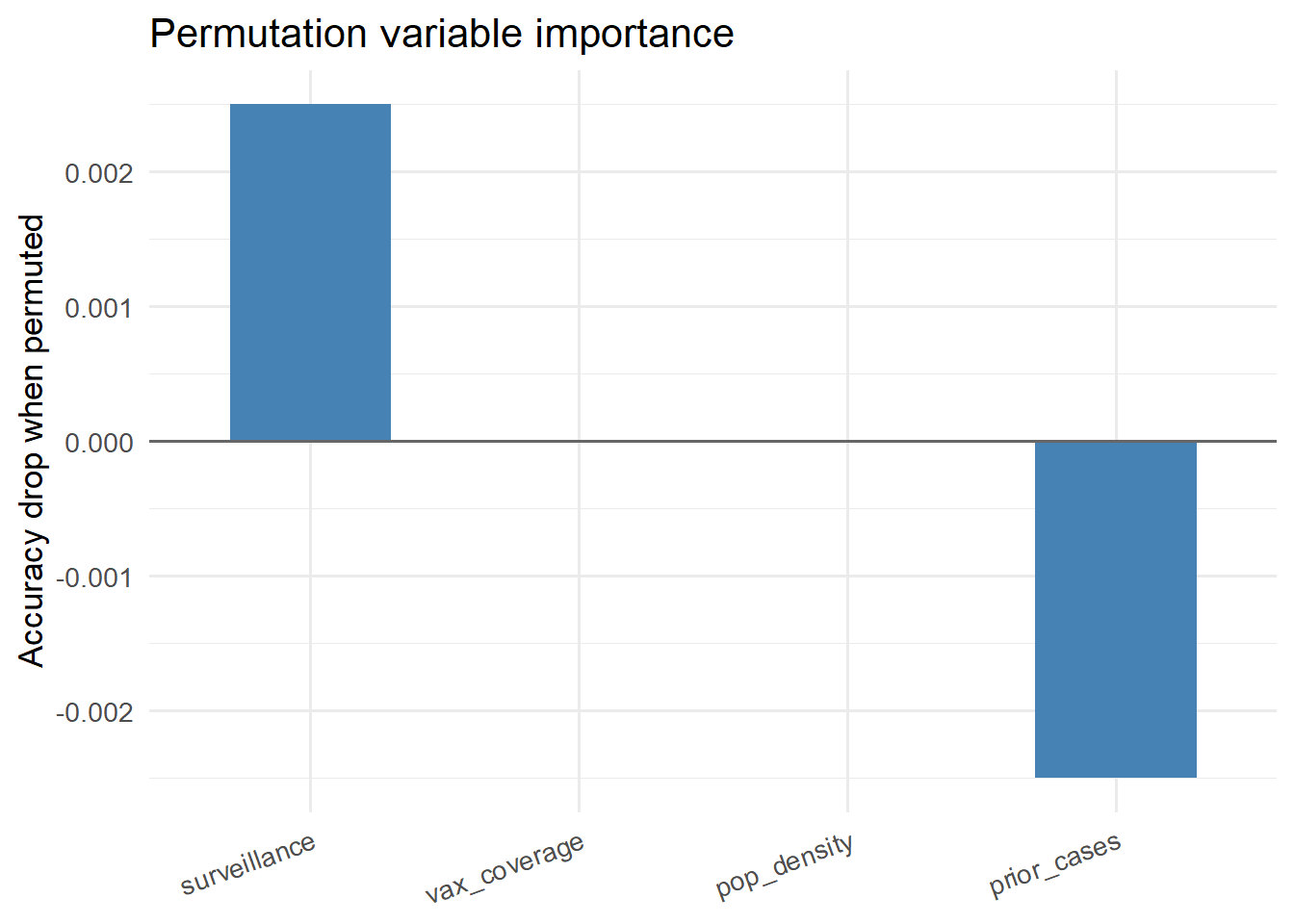
Variable importance via permutation
Permutation importance measures how much accuracy drops when a feature’s values are randomly shuffled — breaking any information it carries (1 ) .
<- mean (bag_predict (forest, df) == df$ outbreak)<- sapply (features, function (feat) {<- df<- sample (df_perm[[feat]]) # shuffle this feature <- mean (bag_predict (forest, df_perm) == df$ outbreak)- acc_perm # drop in accuracy <- data.frame (feature = names (importance),importance = as.numeric (importance)<- imp_df[order (imp_df$ importance, decreasing = TRUE ), ]$ feature <- factor (imp_df$ feature, levels = imp_df$ feature)library (ggplot2)ggplot (imp_df, aes (x = feature, y = importance)) + geom_col (fill = "steelblue" , width = 0.6 ) + geom_hline (yintercept = 0 , colour = "grey40" ) + labs (x = NULL , y = "Accuracy drop when permuted" ,title = "Permutation variable importance" ) + theme_minimal (base_size = 13 ) + theme (axis.text.x = element_text (angle = 20 , hjust = 1 ))
Using ranger in production
The implementation above illustrates the concept. In production, use the ranger package (3 ) , which implements the full algorithm (continuous splits, depth control, proper OOB error estimation) efficiently in C++:
# Production random forest with ranger (eval: false — package may not be installed) library (ranger)<- ranger (~ vax_coverage + pop_density + prior_cases + surveillance,data = df,num.trees = 500 ,mtry = 2 , # features per split (sqrt of total is default) probability = TRUE , # return P(outbreak) not just class importance = "permutation" # Variable importance $ variable.importance# Prediction on new district predict (rf_model, new_district)$ predictions[, "1" ]
Key takeaways
Random forests require almost no tuning — default hyperparameters are competitive on most tabular problems.
They naturally handle missing data, mixed feature types, and non-linear interactions.
Permutation importance is the most reliable variable importance measure because it is model-agnostic.
For outbreak risk scoring with < 10,000 observations, start with a random forest before reaching for a neural network.
References
2.
Hastie T, Tibshirani R, Friedman J. The elements of statistical learning: Data mining, inference, and prediction. 2nd ed. Springer; 2009. doi:
10.1007/978-0-387-84858-7
3.
Wright MN, Ziegler A. Ranger: A fast implementation of random forests for high dimensional data in
C++ and
R . Journal of Statistical Software. 2017;77(1):1–17. doi:
10.18637/jss.v077.i01