Gradient Descent: The Optimization Engine Behind Every ML Model
All of machine learning reduces to minimizing a loss function. Gradient descent does this iteratively — and understanding it unlocks every other ML technique.
machine learning
optimization
R
epidemic modeling
Author
Jong-Hoon Kim
Published
April 24, 2026
1 Why optimization is the heart of ML
Every machine learning algorithm — from linear regression to GPT-4 — is doing the same thing: finding parameter values that minimize a loss function. The loss measures how wrong the model is. Gradient descent is the algorithm that walks downhill on that loss surface to find the minimum.
For an epidemic modeler, this is familiar territory. Fitting a transmission rate \(\beta\) to case data by minimizing sum-of-squared errors is gradient descent — most implementations just call it optim() and hide the mechanics. Understanding those mechanics is what separates someone who uses ML tools from someone who can build and debug them.
2 The algorithm
Given a loss function \(L(\theta)\) over parameters \(\theta\), gradient descent updates parameters each iteration:
where \(\eta\) is the learning rate (step size) and \(\nabla_\theta L\) is the gradient — the direction of steepest ascent. Stepping opposite to the gradient moves downhill.
Three variants differ in how much data each step uses:
Variant
Data per step
Noise
Typical use
Batch GD
Full dataset
Low
Small data, convex losses
Stochastic GD (SGD)
1 sample
High
Online learning
Mini-batch GD
32–512 samples
Medium
Neural networks
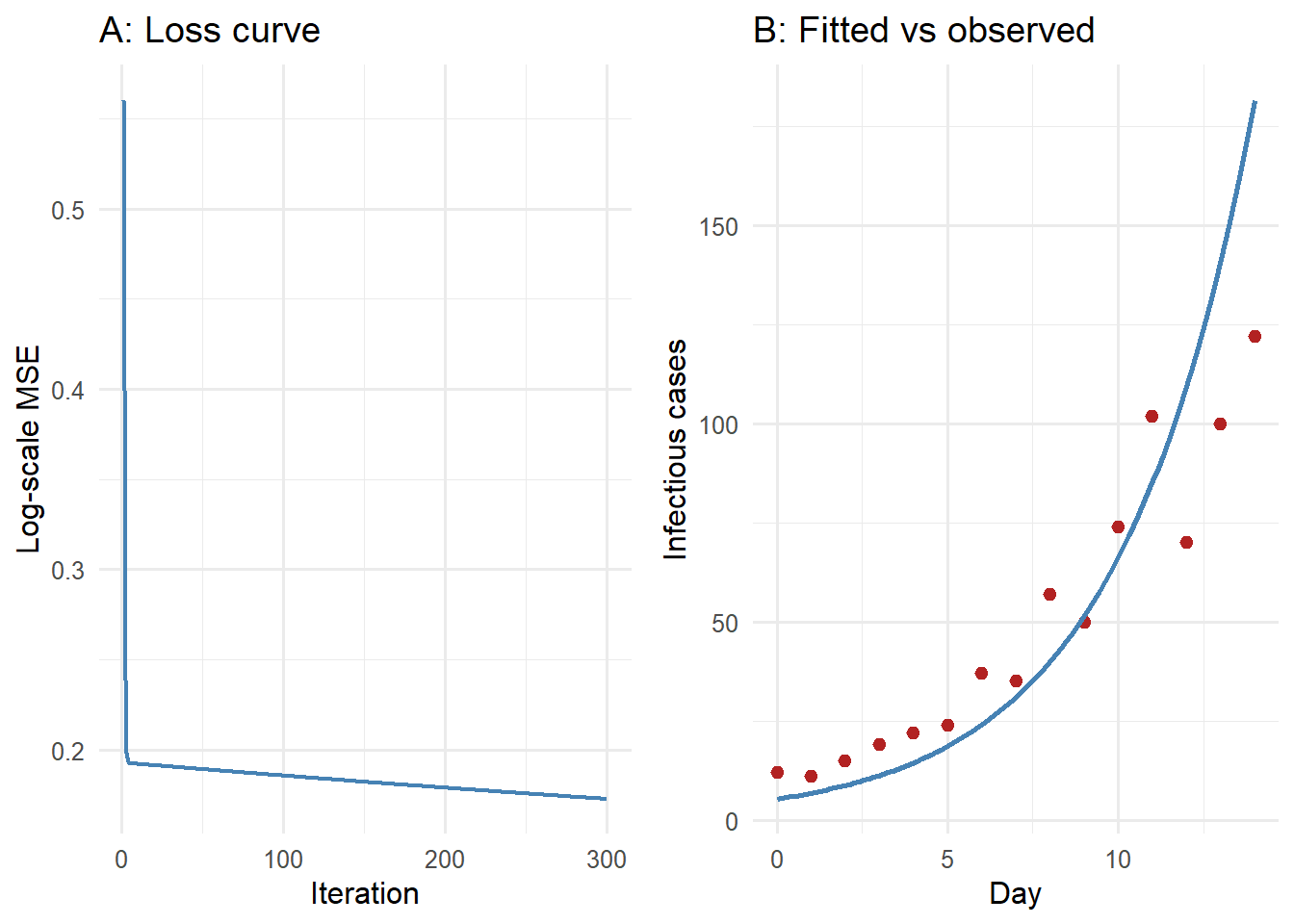
3 From concept to code: fitting an epidemic growth curve
Early epidemic growth is approximately exponential: \(I(t) = I_0 \, e^{rt}\). Given noisy case counts, we want to recover \(I_0\) and \(r\). This is a 2-parameter optimization problem — a clean place to watch gradient descent work.
library(ggplot2)# Panel A: loss curvep_loss <-ggplot(history, aes(x = iter, y = loss)) +geom_line(colour ="steelblue", linewidth =0.8) +labs(x ="Iteration", y ="Log-scale MSE",title ="A: Loss curve") +theme_minimal(base_size =12)# Panel B: fitted vs observedt_fine <-seq(0, 14, length.out =100)I_fit <- params["I0"] *exp(params["r"] * t_fine)df_obs <-data.frame(t = t_obs, cases = I_obs)df_fit <-data.frame(t = t_fine, cases = I_fit)p_fit <-ggplot() +geom_point(data = df_obs, aes(x = t, y = cases),colour ="firebrick", size =2) +geom_line(data = df_fit, aes(x = t, y = cases),colour ="steelblue", linewidth =1) +labs(x ="Day", y ="Infectious cases",title ="B: Fitted vs observed") +theme_minimal(base_size =12)# Side by side with base R layoutgridExtra_available <-requireNamespace("gridExtra", quietly =TRUE)if (gridExtra_available) { gridExtra::grid.arrange(p_loss, p_fit, ncol =2)} else {print(p_loss)print(p_fit)}
Gradient descent convergence. Left: loss falls rapidly in the first 50 iterations then plateaus. Right: the fitted curve closely tracks the observed counts after 300 steps.
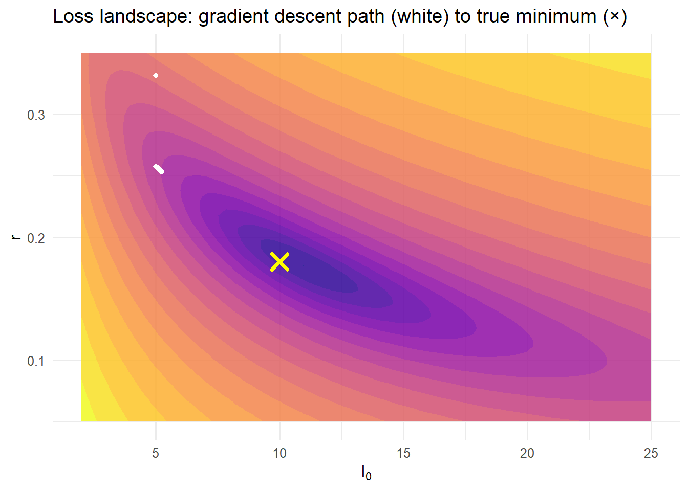
4 The loss landscape: why learning rate matters
The loss surface \(L(I_0, r)\) is a bowl in this case (convex). But in general neural networks have many saddle points and local minima. The learning rate \(\eta\) controls step size:
Too large: parameters overshoot the minimum, loss diverges
Too small: converges correctly but takes thousands of unnecessary iterations
Just right: rapid initial descent, smooth convergence
# Compute loss on a gridI0_grid <-seq(2, 25, length.out =60)r_grid <-seq(0.05, 0.35, length.out =60)grid_df <-expand.grid(I0 = I0_grid, r = r_grid)grid_df$loss <-vapply(seq_len(nrow(grid_df)),function(i) loss(c(grid_df$I0[i], grid_df$r[i])),numeric(1))# Subsample path for readabilitypath_sub <- history[seq(1, n_iter, by =10), ]ggplot(grid_df, aes(x = I0, y = r, z =log(loss +1e-6))) +geom_contour_filled(bins =20, alpha =0.85) +geom_point(data = path_sub, aes(x = I0, y = r, z =NULL),colour ="white", size =1.2) +geom_point(aes(x = I0_true, y = r_true, z =NULL),colour ="yellow", shape =4, size =4, stroke =2) +scale_fill_viridis_d(option ="plasma", guide ="none") +labs(x =expression(I[0]), y ="r",title ="Loss landscape: gradient descent path (white) to true minimum (×)") +theme_minimal(base_size =12)
Loss surface for the epidemic growth parameters (log scale). The gradient descent path (white dots) converges from the starting point (top-left) to the true minimum (center). The contours reveal the elongated valley that makes a fixed learning rate suboptimal — the reason adaptive optimisers like Adam exist.
5 Beyond vanilla gradient descent: Adam
The Adam optimizer (1) adapts the learning rate per parameter using estimates of the first (momentum) and second (variance) moments of the gradient:
# Adam update (conceptual — not executed)m = beta1 * m + (1- beta1) * grad # 1st momentv = beta2 * v + (1- beta2) * grad**2# 2nd momentm_hat = m / (1- beta1**t) # bias correctionv_hat = v / (1- beta2**t)theta = theta - lr * m_hat / (sqrt(v_hat) + eps)
Adam is the default in PyTorch and TensorFlow because it handles elongated loss landscapes (like the one above) much better than fixed-step gradient descent. The default beta1 = 0.9, beta2 = 0.999, lr = 1e-3 work well for most neural networks.
6 What to take away
Gradient descent is not a black box — it is an iterative walk down a loss surface, one parameter update at a time. The practical lessons:
Log-transform count data before computing MSE — raw counts produce loss surfaces that are hard to descend.
Plot your loss curve. If it doesn’t fall, your learning rate is too high or the gradient is broken.
Adam is the safe default for neural networks; optim(method = "L-BFGS-B") is the safe default for low-dimensional epidemic fitting.
Numerical gradients (central differences) let you debug autodiff implementations — if numerical and analytical gradients disagree, your backprop is wrong.
7 References
1.
Kingma DP, Ba J. Adam: A method for stochastic optimization. arXiv preprint arXiv:14126980 [Internet]. 2014. Available from: https://arxiv.org/abs/1412.6980