Self-Attention and Transformers: The Architecture Behind LLMs

Attention is a learned weighted average over past time steps. Build it from scratch in R by solving a concrete prediction task, then see how the full transformer scales the idea.

1 Why transformers matter for epidemic intelligence

“Attention Is All You Need” by Vaswani et al. (1) is likely the most cited paper in the field of deep learning. It introduced the transformer architecture, which rendered recurrent networks obsolete for sequence modeling. The transformer architecture they introduced is now the foundation of every large language model and of the time-series forecasting models emerging in computational epidemiology, including Temporal Fusion Transformer (2) and TimeGPT (3).

Understanding transformers has practical payoffs including the following:

1. Time-series forecasting: attention-based models can learn which past epidemic weeks are most informative for the next-week forecast — something fixed moving averages cannot do.
2. LLM integration: LLMs attend to every part of your prompt when generating each output token. Understanding this mechanism makes you a better prompt engineer.

2 The prediction problem

An epidemic time series has temporal structure: next week’s case count depends on recent weeks, but not all weeks equally. The key question is which past weeks matter most, and by how much.

The simplest forecaster is a moving average (MA): predict next week as the mean of the last \(k\) weeks. This treats all lags equally. Attention learns a weighted average where the weights are optimised to minimise prediction error.

To make this concrete, we generate a 40-week epidemic series and set up a one-step-ahead forecasting task: given the last \(k = 5\) weeks, predict the next week’s case count.

The series is constructed so that both lag 1 and lag 2 carry genuine predictive information. Many respiratory pathogens have an incubation period of roughly two weeks, so today’s reported cases reflect both recent transmission (lag 1) and infections acquired two weeks ago (lag 2). We embed this structure explicitly: the series is the sum of a slow-moving epidemic envelope and a two-week alternating cycle (high week / low week), mimicking a reporting rhythm or biological echo. Lag 2 is in phase with the current week (both land on the same high or low week), while lag 1 is out of phase — making both lags necessary for a good forecast.

set.seed(42)

n     <- 40
t_seq <- 1:n

# Slow-moving epidemic envelope (peaks at week 20)
envelope <- 70 * exp(-((t_seq - 20)^2) / 80) + 15

# 2-week alternating cycle: high/low weeks (reporting rhythm or incubation echo)
biweekly <- 15 * cos(pi * t_seq)   # +15 on odd weeks, -15 on even weeks

# Small AR(1) noise
noise <- numeric(n)
noise[1] <- rnorm(1, 0, 7)
for (t in 2:n) noise[t] <- 0.20 * noise[t - 1] + rnorm(1, 0, 7)

cases <- pmax(1, round(envelope + biweekly + noise))

k <- 5   # look-back window

# Sliding-window dataset: col 1 = lag 1 (most recent), col k = lag k (oldest)
n_pred <- length(cases) - k
X_mat  <- do.call(rbind, lapply(
  (k + 1):length(cases),
  function(i) rev(cases[(i - k):(i - 1)])
))
y_vec  <- cases[(k + 1):length(cases)]

cat("Forecasting steps:", n_pred, "\n")

Forecasting steps: 35 

cat("Observed range:   ", min(cases), "–", max(cases), "cases/week\n")

Observed range:    1 – 105 cases/week

3 Attention as a learned weighted average

A moving average computes \(\hat{y}_t = \frac{1}{k} \sum_{j=1}^{k} x_{t-j}\). Attention generalises this to a softmax-weighted sum:

\[\hat{y}_t = \sum_{j=1}^{k} w_j \, x_{t-j}, \quad \mathbf{w} = \text{softmax}(\boldsymbol{\alpha})\]

where \(\boldsymbol{\alpha} \in \mathbb{R}^k\) are unnormalized attention logits — the parameters we learn. The softmax ensures weights are non-negative and sum to 1. We find \(\boldsymbol{\alpha}\) by minimising mean squared prediction error with gradient descent.

This is the core idea behind every transformer, i.e., learning which positions to attend to. In the following sections, we will see how the idea is generalized to the transformer architecture.

softmax <- function(alpha) {
  e <- exp(alpha - max(alpha))   # numerically stable
  e / sum(e)
}

# Loss: MSE between attention-weighted prediction and true next-week cases
loss_fn <- function(alpha) {
  w    <- softmax(alpha)
  pred <- as.vector(X_mat %*% w)
  mean((pred - y_vec)^2)
}

# Numerical gradient (central differences)
num_grad <- function(f, x, eps = 1e-6) {
  vapply(seq_along(x), function(j) {
    x1 <- x2 <- x
    x1[j] <- x1[j] + eps
    x2[j] <- x2[j] - eps
    (f(x1) - f(x2)) / (2 * eps)
  }, numeric(1))
}

# Gradient descent on alpha
alpha <- rep(0, k)   # start: uniform weights (= moving average)
lr    <- 0.08
for (iter in 1:3000) {
  alpha <- alpha - lr * num_grad(loss_fn, alpha)
}

w_learned <- softmax(alpha)

# Predictions
ma_pred   <- rowMeans(X_mat)                 # baseline: uniform MA
attn_pred <- as.vector(X_mat %*% w_learned)  # attention

# Evaluation
rmse_ma   <- sqrt(mean((ma_pred   - y_vec)^2))
rmse_attn <- sqrt(mean((attn_pred - y_vec)^2))

cat("Learned attention weights (lag 1 = last week, lag 5 = 5 weeks ago):\n")

Learned attention weights (lag 1 = last week, lag 5 = 5 weeks ago):

cat(paste0("  lag ", seq_len(k), ": ", round(w_learned, 3)), sep = "\n")

  lag 1: 0
  lag 2: 0.851
  lag 3: 0
  lag 4: 0.149
  lag 5: 0

cat("\nMoving average RMSE:", round(rmse_ma,   1), "\n")

Moving average RMSE: 21.3 

cat("Attention RMSE:     ", round(rmse_attn, 1), "\n")

Attention RMSE:      13.8 

4 What the learned weights reveal

library(ggplot2)

week_idx <- (k + 1):length(cases)

df_pred <- data.frame(
  week    = rep(week_idx, 3),
  cases   = c(y_vec, ma_pred, attn_pred),
  model   = rep(c("Observed", "Moving avg", "Attention"),
                each = n_pred)
)
df_pred$model <- factor(df_pred$model,
  levels = c("Observed", "Moving avg", "Attention"))

p_pred <- ggplot(df_pred, aes(x = week, y = cases,
                               colour = model, linetype = model)) +
  geom_line(linewidth = 0.9) +
  geom_point(data = subset(df_pred, model == "Observed"),
             size = 1.8) +
  scale_colour_manual(values = c("Observed"    = "black",
                                  "Moving avg"  = "orange",
                                  "Attention"   = "steelblue"),
                      name = NULL) +
  scale_linetype_manual(values = c("Observed"   = "solid",
                                    "Moving avg" = "dashed",
                                    "Attention"  = "solid"),
                        name = NULL) +
  labs(x = "Week", y = "Cases",
       title = "A: One-step-ahead forecast comparison") +
  theme_minimal(base_size = 12) +
  theme(legend.position = "top")

lag_labels <- paste0("lag ", seq_len(k),
                     c(" (last wk)", rep("", k - 1)))
df_weights <- data.frame(
  lag    = factor(lag_labels, levels = lag_labels),
  weight = w_learned
)

p_weights <- ggplot(df_weights, aes(x = lag, y = weight)) +
  geom_col(fill = "steelblue", width = 0.6) +
  geom_hline(yintercept = 1 / k, linetype = "dashed", colour = "firebrick") +
  annotate("text", x = 2, y = 1 / k + 0.03,
           label = "uniform (MA)", colour = "firebrick", size = 3.5) +
  labs(x = "Lag", y = "Attention weight",
       title = "B: Learned attention weights") +
  theme_minimal(base_size = 12) +
  theme(axis.text.x = element_text(angle = 30, hjust = 1))

gridExtra_available <- requireNamespace("gridExtra", quietly = TRUE)
if (gridExtra_available) {
  gridExtra::grid.arrange(p_pred, p_weights, ncol = 2)
} else {
  print(p_pred)
  print(p_weights)
}

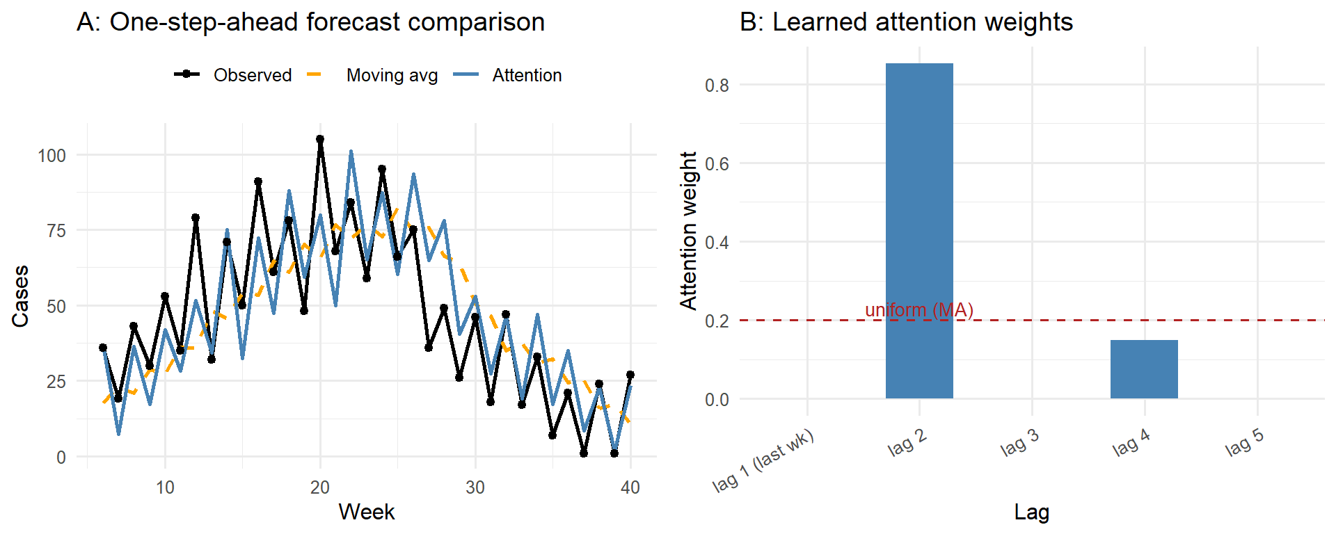
Left: one-step-ahead forecasts. Attention (blue) tracks the epidemic curve more closely than the moving average (orange) by learning non-uniform lag weights. Right: learned attention weights. Lags 2 and 4 (the even lags, in-phase with the 2-week cycle) receive all the weight; lags 1, 3, and 5 (out-of-phase) receive zero. A fixed moving average wastes weight on the out-of-phase lags and is therefore a worse predictor.

The dashed red line in panel B is the uniform weight \(1/k\) that the moving average uses. The learned weights tell a clear story: lags 2 and 4 (the even lags) receive all the weight; lags 1, 3, and 5 receive none. This is the correct discovery — the two-week alternating cycle means every other week is in the same phase as the current week. Lag 1 (one step back) is out of phase: its biweekly component is anti-correlated with the target, so attending to it hurts prediction. The uniform MA does not know this and assigns equal weight to all five lags, averaging in the anti-phase lags and degrading accuracy. Attention finds the phase structure automatically from the data.

5 From weighted average to full self-attention

The predictor above has one limitation: the weights \(\mathbf{w}\) are fixed once trained — they do not adapt to the current value of the sequence. If the epidemic is accelerating versus plateauing, the optimal lag weights differ.

The transformer’s self-attention solves this by making the weights content-dependent. Each position produces a query \(\mathbf{q}\) (“what context am I looking for?”) and keys \(\mathbf{k}_j\) (“what does position \(j\) offer?”). The attention weight from position \(i\) to position \(j\) is:

\[w_{ij} = \frac{\exp(\mathbf{q}_i \cdot \mathbf{k}_j / \sqrt{d_k})}{\sum_j \exp(\mathbf{q}_i \cdot \mathbf{k}_j / \sqrt{d_k})}\]

When the epidemic is growing steeply, the query for the current position will be similar to keys of recent high-growth periods, concentrating weight there. When the epidemic plateaus, the query changes and the attention pattern shifts. This is impossible with a fixed \(\mathbf{w}\).

The full transformer (1) extends further:

Component	Purpose
Multi-head attention	Run \(h\) attention patterns in parallel; different heads may learn short-range vs long-range dependencies
Causal masking	For forecasting, mask future positions so position \(t\) only attends to positions \(\leq t\)
Feed-forward sublayer	Per-position MLP applied after attention (nonlinear feature transform)
Layer normalisation + residuals	Stable training through depth
Positional encoding	Inject position information since attention itself is permutation-invariant

Stack 6–96 such blocks, pre-train on token prediction at scale, and the result is a model that reasons across arbitrarily long contexts — the same mechanism that allows Claude or GPT to follow a 10,000-word prompt consistently.

6 Practical takeaway

• Attention = learned weighted average over context, adapted to content at each position.
• For epidemic forecasting, recent lags deserve higher attention — a fixed MA cannot express this, but learned attention can.
• You do not need to implement a transformer from scratch in production. Use neuralforecast (Python) or Nixtla’s TimeGPT API for transformer-based epidemic forecasting.
• Understanding the mechanism tells you why these models work and what their attention patterns mean when you inspect them.

7 References

1.

Vaswani A, Shazeer N, Parmar N, Uszkoreit J, Jones L, Gomez AN, et al. Attention is all you need. In: Advances in neural information processing systems [Internet]. 2017. Available from: https://arxiv.org/abs/1706.03762

2.

Lim B, Arik SO, Loeff N, Pfister T. Temporal fusion transformers for interpretable multi-horizon time series forecasting. International Journal of Forecasting. 2021;37(4):1748–64. doi:10.1016/j.ijforecast.2021.03.012

3.

Garza A, Challu C, Mergenthaler-Canseco M. TimeGPT-1 [Internet]. arXiv; 2024 [cited 2026 Apr 23]. Available from: https://arxiv.org/abs/2310.03589 doi:10.48550/arXiv.2310.03589