# Parameters
f_val <- 0.5
p_val <- 0.3
r_val <- 0.6
R_seq <- seq(0, 25, length.out = 200)
# Calculate Alpha Star for each R
# We will use numerical optimization for the heterogeneous case to be safe,
# though we could derive the slope sign change.
get_alpha_star_beta <- function(R, f, p, r, nu = 1) {
optim(
par = 0.5, fn = cost_beta,
f = f, p = p, R = R, r = r, nu = nu,
method = "L-BFGS-B", lower = 0, upper = 1
)$par
}
# Wrapper for vector R
calc_curve <- function(R_vec, type) {
sapply(R_vec, function(R) {
if (type == "Homogeneous") {
# Use existing utility
val <- alpha_star_equalrisk(p = p_val, R = R, r = r_val, f = f_val, nu = 1)
# Handle NA (middle region) by 0 or alpha_c ??
# The function returns 0 if reactive is better, alpha_c if mixed is better, 1 if pre.
# It handles the logic.
return(val)
} else {
# Hetero
# Check corners and critical point?
# Numerical is robust
get_alpha_star_beta(R, f_val, p_val, r_val)
}
})
}
df_plot <- data.frame(R = R_seq) %>%
mutate(
Homogeneous = calc_curve(R, "Homogeneous"),
`Beta(1, \\theta)` = calc_curve(R, "Heterogeneous")
) %>%
pivot_longer(cols = c("Homogeneous", "Beta(1, \\theta)"), names_to = "Model", values_to = "Alpha") %>%
group_by(Model) %>%
mutate(
# Create segments for abrupt changes in Homogeneous model
Segment = if (unique(Model) == "Homogeneous") {
cumsum(c(TRUE, abs(diff(Alpha)) > 1e-6))
} else {
1
}
) %>%
ungroup()
# Calculate critical alphas for reference lines
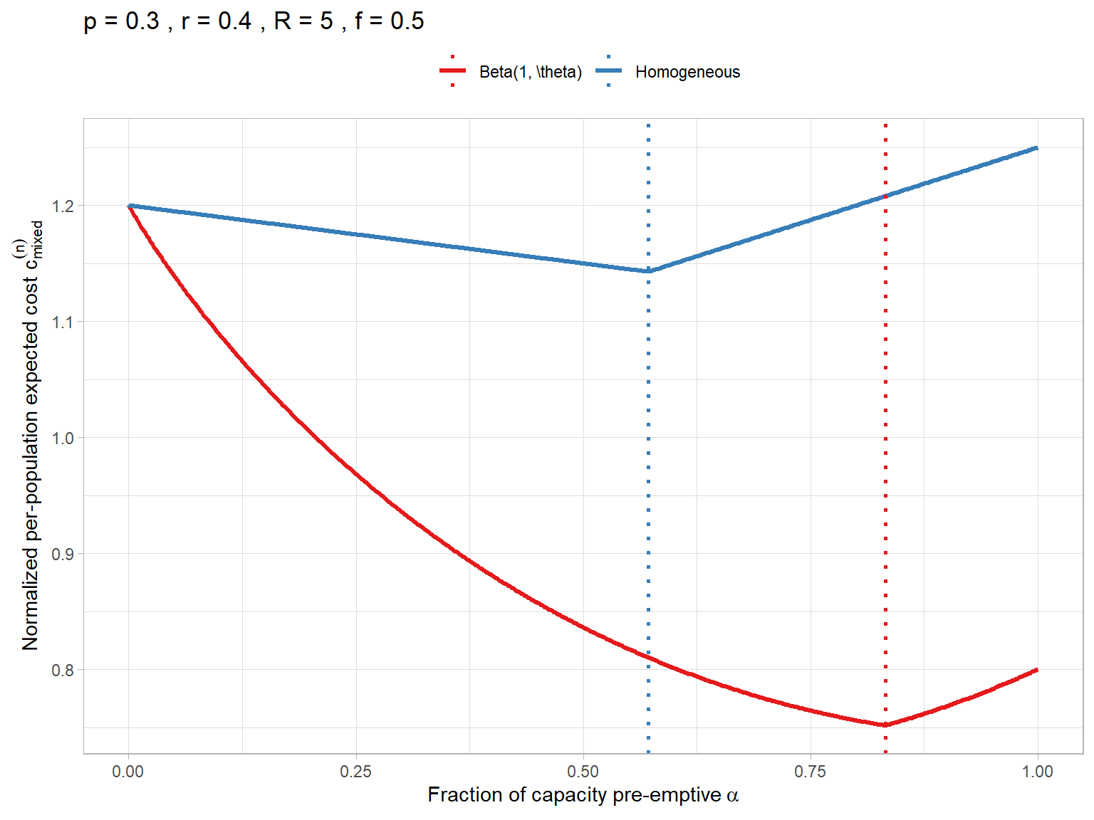
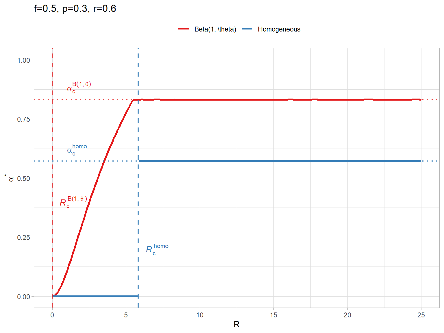
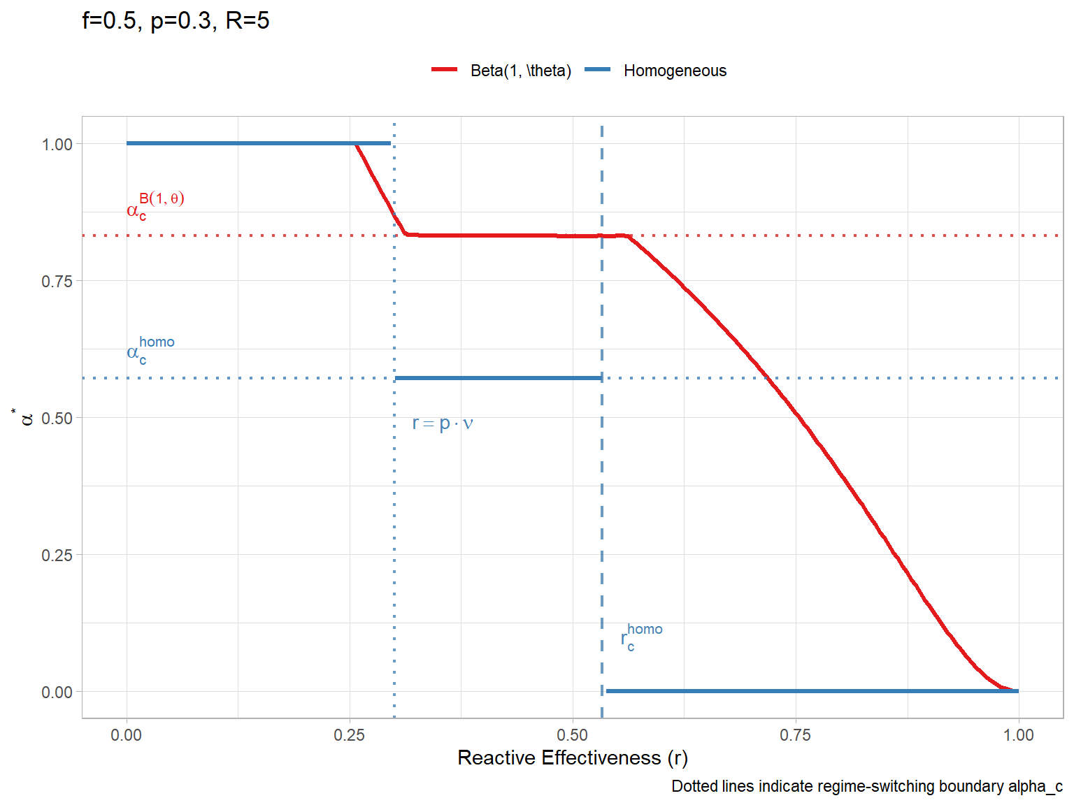
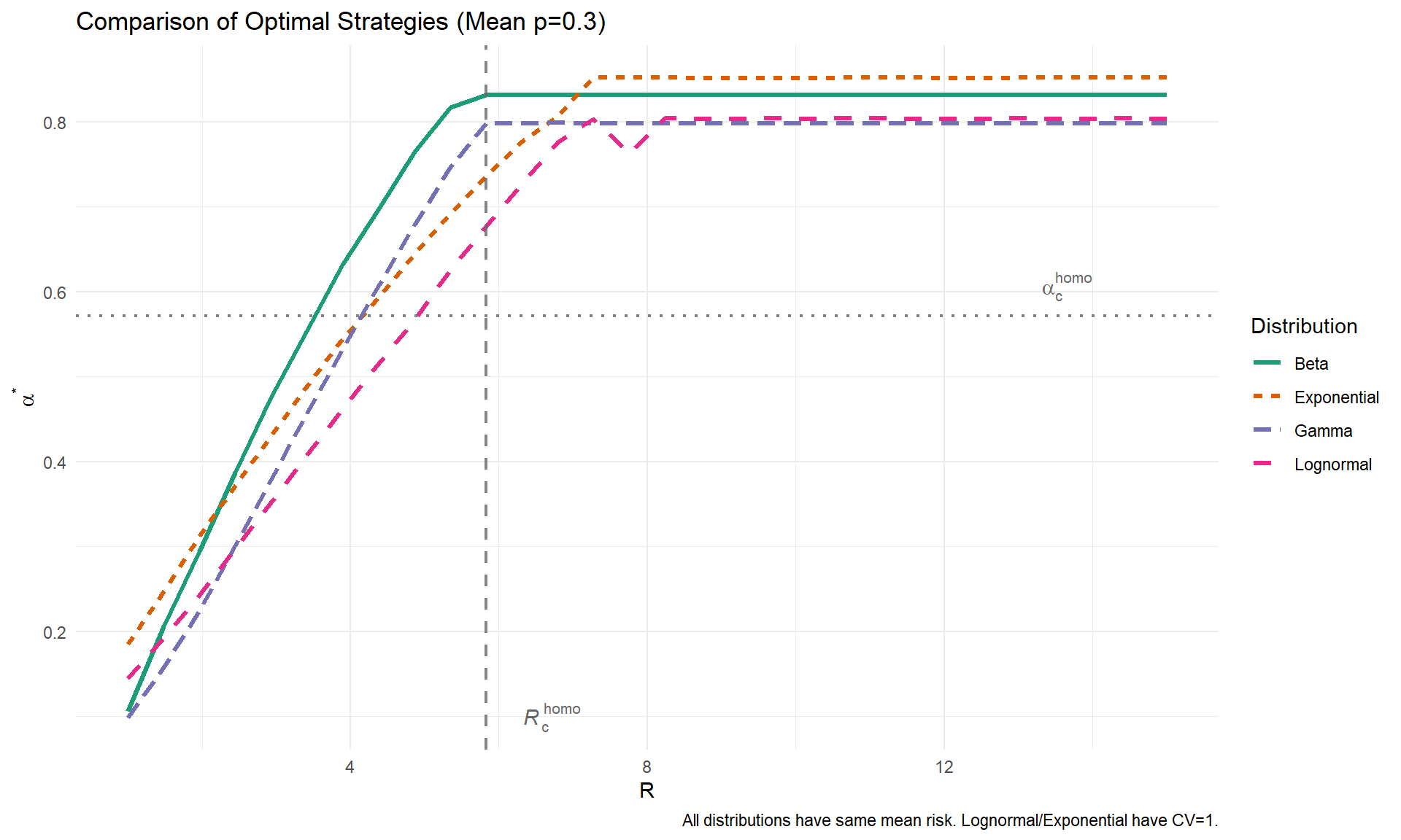
ac_homo <- (f_val - p_val) / (f_val * (1 - p_val))
ac_hetero <- alpha_c_beta(f_val, p_val)
# Calculate critical R (start of pre-emptive vaccination, alpha > 0)
# Homogeneous: R_c = (1-p) / (p * (nu - r)). With nu=1:
Rc_homo <- (1 - p_val) / (p_val * (1 - r_val))
# Heterogeneous: R_c depends on the maximum individual risk x_max.
# R_c = (1 - x_max) / (x_max * (nu - r)).
# For Beta(1, theta), x_max = 1, so Rc_hetero = 0.
Rc_hetero <- 0
df_ref <- data.frame(
Model = c("Homogeneous", "Beta(1, \\theta)"),
Alpha_c = c(ac_homo, ac_hetero),
Label = c("alpha[c]^{homo}", "alpha[c]^{B(1,theta)}")
)
ggplot(df_plot, aes(x = R, y = Alpha, color = Model)) +
geom_line(aes(group = interaction(Model, Segment)), linewidth = 1.2) +
geom_hline(data = df_ref, aes(yintercept = Alpha_c, color = Model), linetype = "dotted", linewidth = 0.8, alpha = 0.8) +
geom_text(data = df_ref, aes(x = 1, y = Alpha_c, label = Label, color = Model), parse = TRUE, hjust = 0, vjust = -0.5, show.legend = FALSE) +
# Add vertical line for Rc (Homogeneous)
geom_vline(xintercept = Rc_homo, linetype = "dashed", color = "#377eb8", linewidth = 0.8, alpha = 0.8) +
annotate("text", x = Rc_homo + 0.5, y = 0.20, label = expression(italic(R)[c]^{
homo
}), parse = TRUE, color = "#377eb8", hjust = 0) +
# Add vertical line for Rc (Beta)
geom_vline(xintercept = Rc_hetero, linetype = "dashed", color = "#e41a1c", linewidth = 0.8, alpha = 0.8) +
annotate("text", x = Rc_hetero + 0.5, y = 0.40, label = expression(italic(R)[c]^{
"B(1," ~ theta ~ ")"
}), parse = TRUE, color = "#e41a1c", hjust = 0) +
theme_light() +
labs(y = expression(alpha^"*"), title = paste0("f=", f_val, ", p=", p_val, ", r=", r_val)) +
scale_color_brewer("", palette = "Set1") +
coord_cartesian(ylim = c(0, 1)) +
theme(legend.position = "top")