---
title: "Minimax: Planning for the Worst-Case Epidemic"
subtitle: "When uncertainty is adversarial, the robust planner plays a zero-sum game against Nature"
author: "Jong-Hoon Kim"
date: "2026-04-20"
categories: [game theory, minimax, robust decision, vaccination, cholera, R]
bibliography: references.bib
csl: https://www.zotero.org/styles/vancouver
format:
html:
toc: true
toc-depth: 3
code-fold: true
code-tools: true
number-sections: true
fig-width: 6
fig-height: 4
fig-align: center
knitr:
opts_chunk:
message: false
warning: false
fig.retina: 2
---
# From Nash to minimax
[The vaccination game](https://www.jonghoonk.com/blog/posts/game_theory_vacc/) was a game between people. Each individual weighed the cost of vaccination against the risk of infection, and the Nash equilibrium emerged from their simultaneous best responses. That framework explains a lot — why voluntary uptake stalls below the herd-immunity threshold, and how large the gap can be.
But at IVI, and in public-health agencies more generally, the operative decision-maker is usually not a pair of strategic individuals. It is a planner — a ministry of health, a WHO technical advisory group, a vaccine-allocation committee — who must commit to a policy before the epidemic unfolds, under substantial uncertainty about what the epidemic will do. The uncertainty can be *parameter* uncertainty ($R_0$, vaccine efficacy, waning), *structural* uncertainty (which compartmental model?), or genuinely *adversarial* (which strain will emerge? where will adherence collapse?).
A useful frame for this is the **game against Nature**. The planner chooses an action; Nature then reveals the state of the world; the planner absorbs the resulting cost. If the planner is risk-neutral and holds a credible prior over Nature's moves, she minimizes expected cost — the **Bayes rule**. If she is unwilling to commit to a prior, or if Nature's move is genuinely adversarial, she minimizes the *worst-case* cost — the **minimax rule**. This post is about the minimax rule: where it comes from, how to compute it, when it is the right thing to do, and when it is not.
# Von Neumann, zero-sum games, and the minimax theorem
Minimax is the oldest result in modern game theory. Von Neumann proved the minimax theorem in 1928 [@vonneumann1928], sixteen years before *Theory of Games and Economic Behavior* and twenty-two years before Nash. Its original setting was the two-player zero-sum game.
Let two players choose mixed strategies $x \in \Delta_n$ and $y \in \Delta_m$ over their respective pure strategies, and let $A$ be an $n \times m$ payoff matrix (Player 1 receives $x^\top A y$; Player 2 receives $-x^\top A y$). Player 1's **maximin** value is what she can guarantee against any opponent:
$$
\underline{v} \;=\; \max_x \min_y\; x^\top A y.
$$
Player 2's **minimax** value is what she can limit her opponent to:
$$
\overline{v} \;=\; \min_y \max_x\; x^\top A y.
$$
It is always true that $\underline{v} \le \overline{v}$. **Von Neumann's minimax theorem** asserts that for finite zero-sum games played in mixed strategies, equality holds:
$$
\underline{v} \;=\; \overline{v} \;=\; v, \tag{1}
$$
and the common value $v$ is the **value of the game**. Pure-strategy equilibria can fail to exist — rock–paper–scissors has none — but mixed-strategy equilibria always do. Existence is proved via the separating-hyperplane theorem (equivalently, LP duality); it was the first equilibrium existence result in game theory and a precursor to Nash's 1950 theorem for general $n$-player games [@nash1950].
The key link back to Part 1: **in two-player zero-sum games, Nash equilibrium, minimax, and maximin all coincide**. Outside this class — including the vaccination game, which is non-zero-sum and has externalities — they generally differ.
::: {.callout-tip}
## What you need
```r
install.packages(c("dplyr", "tidyr", "ggplot2", "patchwork", "truncnorm"))
```
Code tested with: R 4.4, `ggplot2 3.5`, `dplyr 1.1`.
:::
---
# Minimax as a decision rule
Wald [@wald1950] generalised minimax from game theory to statistical decision theory. Consider a decision-maker choosing action $a$ in a space $\mathcal{A}$, facing an unknown state of nature $\theta \in \Theta$, with loss $L(a, \theta)$. Three canonical rules deserve their names:
| Rule | Formula | When it is the right thing |
| --- | --- | --- |
| **Bayes** | $a_B \;=\; \arg\min_a \int L(a, \theta)\, \pi(\theta)\, d\theta$ | We trust the prior $\pi$ |
| **Minimax** | $a_M \;=\; \arg\min_a \sup_{\theta \in \Theta} L(a, \theta)$ | We do not trust the prior; Nature is (or might as well be) adversarial |
| **Minimax regret** | $a_R \;=\; \arg\min_a \sup_\theta \big\{ L(a, \theta) - \min_{a'} L(a', \theta) \big\}$ | We want to minimise *opportunity loss* rather than absolute loss |
Minimax is often criticised as **pessimistic**: it hedges against states of nature that may be vanishingly improbable. For an infectious-disease planner, this can mean hedging against $R_0 = 15$ in a setting where credible estimates place $R_0$ in $[2, 4]$. The remedy is not to abandon minimax but to **restrict the uncertainty set** $\Theta$ — a device called **$\Gamma$-minimax** when $\Gamma$ is a family of priors rather than a set of parameters [@berger1985]. We return to this at the end.
---
# The minimax vaccination problem
Let us ground the abstraction in a problem close to our work at IVI: a cholera-prone setting where oral cholera vaccine (OCV) must be allocated before outbreak onset, under uncertainty about transmissibility. We will compute the minimax coverage $\pi_{\text{mm}}$ and compare it against two references — a Bayes-optimal coverage $\pi_{B}$ and the Nash coverage $\pi^*$ from Part 1.
## Setup
Fix an SIR model with a perfect pre-epidemic vaccine, coverage $\pi$, and basic reproduction number $R_0$. Among the unvaccinated, the attack fraction $w$ satisfies the classical final-size relation
$$
w \;=\; 1 - \exp\!\big(-R_0\,(1 - \pi)\,w\big), \tag{2}
$$
with $w = 0$ whenever $R_0(1 - \pi) \le 1$. The population-level attack rate is $\text{AR}(\pi, R_0) = (1-\pi)\, w$. We take the planner's per-capita loss as
$$
L(\pi, R_0) \;=\; c_v \cdot \pi \;+\; c_i \cdot \text{AR}(\pi, R_0), \tag{3}
$$
where $c_v$ is the per-dose vaccination cost and $c_i$ is the per-case cost (DALYs, economic loss, …). The only uncertainty is over $R_0$, which lies in $[R_{\min}, R_{\max}]$.
## Implementation
```{r}
#| label: setup
library(dplyr)
library(tidyr)
library(ggplot2)
library(patchwork)
library(truncnorm)

theme_set(
    theme_minimal(base_size = 10) +
        theme(
            panel.grid.minor = element_blank(),
            plot.title       = element_text(face = "bold", size = 10),
            legend.position  = "bottom"
        )
)

C_NASH <- "#F44336" # red
C_SOCIAL <- "#2196F3" # blue
C_CRIT <- "#4CAF50" # green
C_MINIMAX <- "#FF9800" # orange
C_GAP <- "#9C27B0" # purple
```
```{r}
#| label: core-functions
# Attack rate from the SIR final-size relation (perfect pre-vaccination)
attack_rate <- function(pi, R0) {
    Reff <- R0 * (1 - pi)
    if (Reff <= 1) {
        return(0)
    }
    w <- uniroot(
        \(w) w - (1 - exp(-Reff * w)),
        interval = c(1e-8, 1 - 1e-8)
    )$root
    (1 - pi) * w
}

# Planner's per-capita loss
loss <- function(pi, R0, cv = 0.10, ci = 1.0) {
    cv * pi + ci * attack_rate(pi, R0)
}

# Worst-case loss over R0 in [R_lo, R_hi]
worst_case <- function(pi, R_lo, R_hi, cv, ci) {
    R_grid <- seq(R_lo, R_hi, length.out = 60)
    max(sapply(R_grid, \(R0) loss(pi, R0, cv, ci)))
}

# Minimax coverage: minimises the worst-case loss
minimax_pi <- function(R_lo, R_hi, cv = 0.10, ci = 1.0) {
    optimize(\(pi) worst_case(pi, R_lo, R_hi, cv, ci),
        interval = c(0, 1)
    )$minimum
}

# Bayes coverage: minimises expected loss under a truncated-normal prior
bayes_pi <- function(R0_mean, R0_sd, R_lo = 1.1, R_hi = 20,
                     cv = 0.10, ci = 1.0, n = 500) {
    R0_samples <- rtruncnorm(n,
        a = R_lo, b = R_hi,
        mean = R0_mean, sd = R0_sd
    )
    optimize(
        \(pi) mean(sapply(R0_samples, \(R0) loss(pi, R0, cv, ci))),
        interval = c(0, 1)
    )$minimum
}

# Nash coverage from Part 1 (linear pi_inf)
nash_coverage <- function(R0, q, r) {
    pi_c <- 1 - 1 / R0
    if (r >= q) {
        return(0)
    }
    uniroot(
        \(pi) q * pmax(0, 1 - pi / pi_c) - r,
        interval = c(0, pi_c)
    )$root
}
```
## A worked example
Take the uncertainty set $R_0 \in [1.5, 6]$ — a range spanning published cholera estimates across endemic and outbreak settings. Set $c_v = 0.10$ and $c_i = 1$ (a single dose costs 10% of an averted case), and place a Bayesian prior centred at $R_0 = 2.5$ with standard deviation $0.8$.
```{r}
#| label: three-strategies
R_lo <- 1.5
R_hi <- 6
cv <- 0.10
ci <- 1.0

pi_mm <- minimax_pi(R_lo, R_hi, cv, ci)
pi_B <- bayes_pi(
    R0_mean = 2.5, R0_sd = 0.8,
    R_lo = R_lo, R_hi = R_hi, cv = cv, ci = ci
)
pi_N <- nash_coverage(R0 = 2.5, q = 0.5, r = 0.10)

tibble(
    strategy = c(
        "Nash equilibrium (pi*, from Part 1)",
        "Bayes-optimal (pi_B)",
        "Minimax (pi_mm)",
        "Herd-immunity threshold at R_max"
    ),
    value = c(pi_N, pi_B, pi_mm, 1 - 1 / R_hi)
) |>
    mutate(value = sprintf("%.3f", value)) |>
    knitr::kable()
```
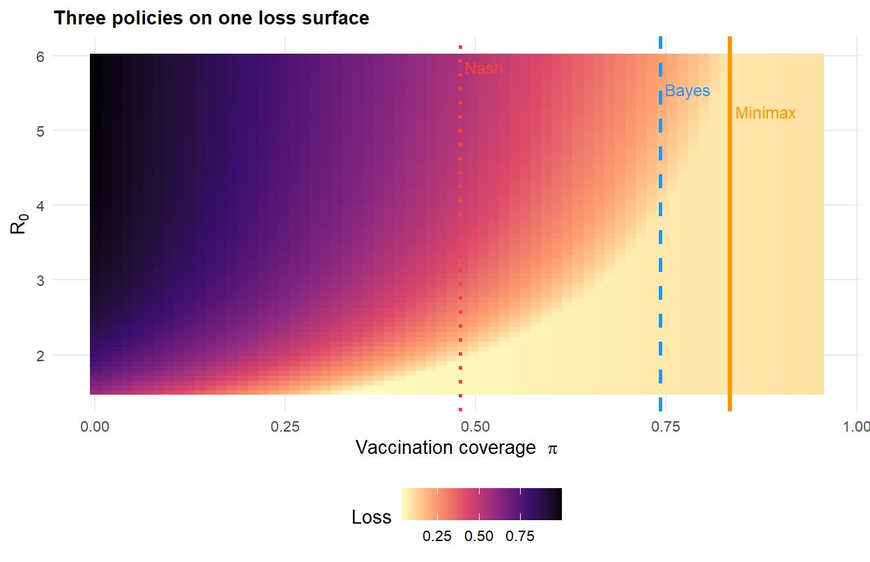
The pattern is what the theory anticipates. Voluntary uptake (Nash) is lowest — individuals free-ride on the herd. The Bayes planner does better, pulling coverage upward to internalise the externality. The minimax planner does *more*, pushing coverage close to the herd-immunity threshold of the worst-case $R_0$ in the uncertainty set.
## An analytical short-cut
Because $L(\pi, R_0)$ is monotone increasing in $R_0$ whenever $\pi < 1 - 1/R_0$, the inner supremum in the minimax problem is attained at $R_0 = R_{\max}$:
$$
\pi_{\text{mm}} \;=\; \arg\min_\pi\, L(\pi, R_{\max}). \tag{4}
$$
**The minimax planner acts as if $R_0$ were pinned at its upper bound and ignores everything else.** This is simultaneously minimax's strength — it is robust to misspecification of the prior — and its weakness. It can demand expensive hedging against very unlikely scenarios.
## Visualising the loss surface
```{r}
#| label: loss-surface
#| fig-cap: "Planner's loss as a function of coverage $\\pi$ and $R_0$, with three candidate policies overlaid. The minimax policy is pinned to the worst-case $R_0 = 6$; the Bayes policy responds to the full prior; the Nash coverage ignores the externality entirely."
#| fig-width: 6.5
#| fig-height: 4.2
grid <- expand_grid(
    pi = seq(0, 0.95, length.out = 70),
    R0 = seq(R_lo, R_hi, length.out = 70)
) |>
    rowwise() |>
    mutate(L = loss(pi, R0, cv, ci)) |>
    ungroup()

ggplot(grid, aes(x = pi, y = R0, fill = L)) +
    geom_raster() +
    scale_fill_viridis_c(option = "magma", direction = -1, name = "Loss") +
    geom_vline(xintercept = pi_N, colour = C_NASH, linewidth = 1.0, linetype = "dotted") +
    geom_vline(xintercept = pi_B, colour = C_SOCIAL, linewidth = 1.0, linetype = "dashed") +
    geom_vline(xintercept = pi_mm, colour = C_MINIMAX, linewidth = 1.1) +
    annotate("text", x = pi_N, y = R_hi - 0.15, label = "Nash", hjust = -0.1, colour = C_NASH, size = 3.2) +
    annotate("text", x = pi_B, y = R_hi - 0.45, label = "Bayes", hjust = -0.1, colour = C_SOCIAL, size = 3.2) +
    annotate("text", x = pi_mm, y = R_hi - 0.75, label = "Minimax", hjust = -0.1, colour = C_MINIMAX, size = 3.2) +
    labs(
        x = expression("Vaccination coverage  " * pi),
        y = expression(R[0]),
        title = "Three policies on one loss surface"
    )
```
## How the policies respond to the width of the uncertainty set
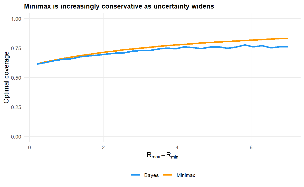
The most revealing comparison is over the *width* of the uncertainty set. A Bayesian planner tracks the mean of the prior; a minimax planner tracks its upper bound.
```{r}
#| label: uncertainty-width
#| fig-cap: "Optimal coverage as a function of the width of the uncertainty set, centred on $R_0 = 2.5$. The minimax policy scales with the upper bound of the set; the Bayes policy is largely driven by the mean."
#| fig-width: 6.5
#| fig-height: 4
R0_centre <- 2.5
widths <- seq(0.2, 7, length.out = 30)

sweep <- tibble(
    width = widths,
    R_lo  = pmax(1.1, R0_centre - widths / 2),
    R_hi  = R0_centre + widths / 2
) |>
    rowwise() |>
    mutate(
        pi_minimax = minimax_pi(R_lo, R_hi, cv, ci),
        pi_bayes = bayes_pi(
            R0_centre, pmax(widths / 4, 0.05),
            R_lo, R_hi, cv, ci
        )
    ) |>
    ungroup()

ggplot(sweep, aes(x = width)) +
    geom_line(aes(y = pi_minimax, colour = "Minimax"), linewidth = 1.1) +
    geom_line(aes(y = pi_bayes, colour = "Bayes"), linewidth = 1.1) +
    scale_colour_manual(
        values = c(Minimax = C_MINIMAX, Bayes = C_SOCIAL),
        name = NULL
    ) +
    labs(
        x = expression(R[max] - R[min]),
        y = "Optimal coverage",
        title = "Minimax is increasingly conservative as uncertainty widens"
    ) +
    coord_cartesian(ylim = c(0, 1))
```
When the uncertainty set is narrow the two policies agree. As it widens, the minimax policy pulls sharply upward, tracking the worst plausible $R_0$, while the Bayes policy stays close to the prior mean. Which is appropriate depends on how much trust the prior deserves.
---
# Host–pathogen games: two caveats
It is tempting to describe host-pathogen interactions as minimax games: the pathogen "wants" to maximise spread; the host "wants" to minimise it. Some of the formal machinery transfers usefully — ESS analysis uses fixed-point arguments that echo minimax — but the analogy needs two caveats.
**(1) Pathogens do not optimise.** Evolution by natural selection produces strategies that are evolutionarily stable *given the current environment*, but it does not anticipate or counter-select. A strict minimax frame in which the pathogen chooses the worst case for the host typically over-states what evolution can do.
**(2) The game is rarely zero-sum.** Virulence–transmissibility trade-offs [@anderson1982; @alizon2009] show that a more virulent strain can be bad for both pathogen persistence and host welfare — the pathogen's payoff is not a simple negation of the host's.
That said, two minimax-like frames are genuinely useful for pathogen-evolution problems:
- **Robust vaccine design.** The planner chooses a vaccine whose efficacy must hold across a set of circulating strains. This is minimax in antigen space, used in seasonal influenza vaccine composition and — increasingly — for typhoid Vi-TCV against potential Vi-negative escape.
- **Adversarial simulation.** In outbreak-response planning, we often stress-test policies against a "red team" parameter choice. That is minimax in practice, even when it is not named as such.
A fuller treatment of evolutionary games awaits Post 4.
---
# Minimax outside of game theory
Minimax has made a second career outside game theory, and three instances are worth knowing if you build models at the interface of epidemiology and machine learning.
**Distributionally robust optimisation (DRO).** Rather than minimise expected loss under a fixed data distribution, one minimises expected loss under the *worst-case distribution within a divergence ball* around the empirical distribution [@benTal2009; @duchi2021]:
$$
\hat\theta \;=\; \arg\min_\theta\; \sup_{Q\,:\, D(Q\,\|\,\hat P)\, \le\, \rho}\; \mathbb{E}_Q\big[L(\theta, X)\big]. \tag{5}
$$
For fitting disease models to outbreak data, DRO is a principled guard against covariate shift between the training setting and the deployment setting.
**Adversarial training.** A neural-network classifier is trained against worst-case small perturbations of its inputs [@goodfellow2015]:
$$
\min_\theta\, \mathbb{E}_{(x,y)}\!\Big[\, \max_{\|\delta\| \le \epsilon}\, L\big(f_\theta(x + \delta),\, y\big)\,\Big]. \tag{6}
$$
This is a standard ingredient when building diagnostic models that must be robust to slight image-acquisition differences across sites.
**Minimax-weighted PINN training.** A physics-informed neural network fits data loss and PDE-residual loss jointly. Several recent papers recast the balancing of the two loss terms as a minimax problem — the network minimising while a dual variable maximises across collocation points — and find that this stabilises training and improves out-of-distribution generalisation [@mcclenny2023]. The frame is of direct interest for PINN-based epidemic reconstruction.
The common thread is that **minimax is what we reach for when we want guarantees in the presence of something we cannot control or cannot model** — an unobserved parameter, a distributional shift, a crafted perturbation, or (in game theory proper) a strategic opponent.
---
# When minimax is too pessimistic
Pure minimax has three well-known pathologies, each with a standard remedy.
| Pathology | Remedy |
| --- | --- |
| Hedges against vanishingly improbable states | **$\Gamma$-minimax**: optimise over the worst prior in a restricted family $\Gamma$ |
| Ignores the *margin* by which other actions are worse in good states | **Minimax regret** [@savage1951] |
| Changes sharply when the uncertainty set is expanded | **Smooth ambiguity** [@klibanoff2005] |
For OCV allocation in particular, minimax *regret* is often the more defensible frame: *how much worse could I be, relative to the best policy in hindsight?* It produces less cautious — and more communicable — recommendations than pure minimax.
---
# What the minimax frame tells us
| Question | Answer |
| --- | --- |
| Does minimax coincide with Nash? | Only in 2-player zero-sum games. |
| Does minimax depend on a prior? | No — that is its virtue, and its cost. |
| Is the minimax planner "rational"? | Rational in the Wald sense; often over-cautious in the Bayesian sense. |
| When should an epidemiologist reach for it? | When the uncertainty set is plausibly broad, the consequences of underestimating it are severe, and no credible prior is available. |
| When should an epidemiologist avoid it? | When expert priors are well-calibrated and decision-relevant. |
| What is the operational short-cut? | For monotone losses, the minimax planner optimises at the worst-case parameter. |
---
# Series roadmap
1. **[Foundations.](https://www.jonghoonk.com/blog/posts/game_theory_vacc/)** Vaccination game, Nash equilibrium, social optimum, price of anarchy.
2. **(This post) Minimax and the adversarial planner.** Von Neumann's theorem, Wald decision theory, worst-case OCV allocation, connections to DRO and PINN robustness.
3. **Coupled behaviour–disease dynamics.** Replicator and imitation dynamics layered onto SIR models.
4. **Evolutionary game theory for pathogens.** Virulence–transmissibility trade-offs, ESS analysis, strain replacement under vaccination pressure — with cholera and typhoid as running examples.
5. **Policy and mechanism design.** Subsidies, mandates, information campaigns, network games, and agentic LLM-driven decision models.
---
# References {.unnumbered}
::: {#refs}
:::
```{r}
#| label: session-info
#| echo: false
cat(sprintf("R %s\n", paste(R.version$major, R.version$minor, sep = ".")))
for (pkg in c("ggplot2", "dplyr", "tidyr", "patchwork", "truncnorm")) {
cat(sprintf("%-10s %s\n", pkg, as.character(packageVersion(pkg))))
}
```