seir_step <- function(state, beta, sigma, gamma, dt = 1.0) {
S <- max(0, state["S"], na.rm = TRUE)
E <- max(0, state["E"], na.rm = TRUE)
I <- max(0, state["I"], na.rm = TRUE)
R <- max(0, state["R"], na.rm = TRUE)
if (!is.finite(beta) || beta <= 0) beta <- 0.001
N <- S + E + I + R
if (!is.finite(N) || N <= 0) {
return(c(S = 0, E = 0, I = 0, R = 0, deltaI = 0))
}
new_exp <- beta * S * I / N * dt
new_inf <- sigma * E * dt
new_rec <- gamma * I * dt
c(
S = S - new_exp,
E = E + new_exp - new_inf,
I = I + new_inf - new_rec,
R = R + new_rec,
deltaI = new_inf # observed: new infections
)
}Real-Time State Estimation with the Ensemble Kalman Filter
Updating an epidemic model as data arrive — from the classic KF to the nonlinear ensemble version. Post 4 in the Building Digital Twin Systems series.
digital twin
Kalman filter
data assimilation
R
epidemic modeling
1 The gap between a model and a digital twin
An epidemic model fed fixed parameters produces a single trajectory. A digital twin does something more: it continuously updates its internal state as real data arrive, so that at every point in time the model reflects the current best estimate of reality.
The standard Kalman filter (1) achieves this for linear systems. An SIR model is nonlinear — transmission depends on the product \(SI\), not a sum. The Ensemble Kalman Filter (EnKF) (2,3) extends the idea to nonlinear models by representing uncertainty through a cloud of particles (an ensemble) rather than an analytical covariance matrix. It was first applied to epidemic forecasting for influenza by Shaman et al. (4) and is now a core tool for real-time surveillance.
2 The Kalman filter idea
The Kalman filter alternates two steps.
Forecast step — propagate the current state estimate forward using the model: \[\hat{x}_t^- = f(\hat{x}_{t-1})\] \[P_t^- = F P_{t-1} F^\top + Q\] where \(P\) is the error covariance, \(F\) is the linearised model Jacobian, and \(Q\) is process noise.
Update step — correct the forecast using a new observation \(y_t\): \[K_t = P_t^- H^\top (H P_t^- H^\top + R)^{-1}\] \[\hat{x}_t = \hat{x}_t^- + K_t(y_t - H \hat{x}_t^-)\] \[P_t = (I - K_t H) P_t^-\]
\(H\) maps the model state to the observation space, \(R\) is observation noise, and \(K\) is the Kalman gain — a weight that balances model uncertainty against observation uncertainty.
The EnKF replaces the analytical \(P\) with a sample covariance computed from an ensemble of \(N\) model runs.
3 The EnKF algorithm
Initialise: draw N particles from the prior
For each observation time t:
  1. FORECAST: propagate each particle through the model
  2. ANALYSE:
     a. Compute ensemble mean and sample covariance P
     b. For each particle i, add observation noise: ỹᵢ = y_t + ε_i, ε_i ~ N(0, R)
     c. Compute Kalman gain: K = P Hᵀ (H P Hᵀ + R)⁻¹
     d. Update each particle: xᵢ ← xᵢ + K(ỹᵢ - H xᵢ)
The perturbed observations in step 2b prevent ensemble collapse (all particles converging to the same point) and preserve the theoretical covariance relationship (3).
4 Implementation in R
We use an SEIR model: \(S \to E \to I \to R\), where \(E\) is a latent exposed compartment with mean duration \(1/\sigma\). The observed variable is the new infectious count \(\Delta I\) (newly symptomatic cases per day), not the total \(I\) — matching real surveillance data.
4.1 The process model
4.2 Generating synthetic observations
We simulate a “true” outbreak and observe daily new cases with Poisson noise — a common model for reported case counts.
set.seed(42)

# True parameters
N_pop   <- 100000
beta_t  <- 0.35
sigma_t <- 1 / 5   # incubation 5 days
gamma_t <- 1 / 7   # infectious 7 days

# Simulate true trajectory
true_state <- c(S = N_pop - 50, E = 30, I = 20, R = 0, deltaI = 0)
n_days <- 90
true_traj <- matrix(0, nrow = n_days + 1, ncol = 5)
colnames(true_traj) <- names(true_state)
true_traj[1, ] <- true_state

for (d in seq_len(n_days)) {
  true_traj[d + 1, ] <- seir_step(true_traj[d, ],
                                   beta_t, sigma_t, gamma_t)
}

# Observed: Poisson noise on new infections
obs <- rpois(n_days, lambda = pmax(1, true_traj[-1, "deltaI"]))library(ggplot2)
days <- 0:n_days
df_truth <- data.frame(
day = days,
S = true_traj[, "S"],
E = true_traj[, "E"],
I = true_traj[, "I"],
R = true_traj[, "R"]
)
ggplot(df_truth, aes(x = day)) +
geom_line(aes(y = E, colour = "Exposed")) +
geom_line(aes(y = I, colour = "Infectious")) +
geom_point(data = data.frame(day = seq_len(n_days), obs = obs),
aes(x = day, y = obs, colour = "Observed"),
size = 0.8, alpha = 0.7) +
scale_colour_manual(values = c(Exposed = "orange",
Infectious = "firebrick",
Observed = "grey40")) +
labs(x = "Day", y = "Count", colour = NULL) +
theme_minimal(base_size = 13)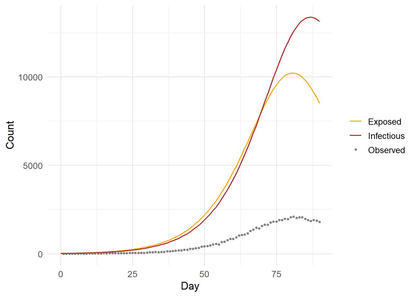
4.3 The EnKF function
enkf_seir <- function(obs,           # vector of daily observations
                      N_pop,         # population size
                      N_ens = 200,   # ensemble size
                      sigma = 1/5,   # fixed incubation rate
                      gamma = 1/7,   # fixed recovery rate
                      beta_mean = 0.3,
                      beta_sd   = 0.1,
                      obs_var   = NULL) {

  n_obs   <- length(obs)
  # State vector: (S, E, I, R, log_beta)
  # log_beta is estimated alongside states
  n_state <- 5

  # Initialise ensemble from prior
  ens <- matrix(0, nrow = N_ens, ncol = n_state)
  colnames(ens) <- c("S", "E", "I", "R", "log_beta")

  # Spread initial infections across S and I
  I_init      <- round(rnorm(N_ens, 20, 5))
  I_init      <- pmax(I_init, 1)
  ens[, "I"]  <- I_init
  ens[, "S"]  <- N_pop - I_init
  ens[, "E"]  <- 0
  ens[, "R"]  <- 0
  ens[, "log_beta"] <- rnorm(N_ens, log(beta_mean), beta_sd)

  # Containers for posterior summaries
  beta_post <- matrix(NA, nrow = n_obs, ncol = 3)  # median, q2.5, q97.5
  I_post    <- matrix(NA, nrow = n_obs, ncol = 3)
  deltaI_post <- matrix(NA, nrow = n_obs, ncol = 3)

  for (t in seq_len(n_obs)) {

    # Sanitise ensemble before forecast: replace any NaN/Inf with safe values
    for (col in c("S", "E", "I", "R")) {
      bad <- !is.finite(ens[, col])
      ens[bad, col] <- 0
    }
    bad_lb <- !is.finite(ens[, "log_beta"])
    ens[bad_lb, "log_beta"] <- log(beta_mean)

    # --- 1. Forecast ---
    beta_ens <- exp(ens[, "log_beta"])
    state_names <- c("S", "E", "I", "R", "deltaI")
    forecast_ens <- matrix(0, nrow = N_ens, ncol = 5)
    colnames(forecast_ens) <- state_names

    for (i in seq_len(N_ens)) {
      st_vals <- pmax(0, ens[i, c("S", "E", "I", "R")])
      st_vals[!is.finite(st_vals)] <- 0
      st <- c(S = st_vals[1], E = st_vals[2],
              I = st_vals[3], R = st_vals[4], deltaI = 0)
      forecast_ens[i, ] <- seir_step(st, beta_ens[i], sigma, gamma)
    }

    # Add random walk noise to log_beta (model evolution)
    ens[, "log_beta"] <- ens[, "log_beta"] + rnorm(N_ens, 0, 0.02)

    # Update states from forecast
    ens[, c("S","E","I","R")] <- forecast_ens[, c("S","E","I","R")]
    ens[, ] <- pmax(ens, 0)   # keep non-negative

    # --- 2. Analyse ---
    # Observation operator H: maps state → observed deltaI
    H_vec <- forecast_ens[, "deltaI"]   # one observation per particle

    # Observation noise variance
    obs_r <- if (is.null(obs_var)) max(obs[t], 1) else obs_var

    # Ensemble covariance of (state, Hy)
    state_full <- cbind(ens[, c("S","E","I","R")],
                        log_beta = ens[, "log_beta"])
    ensemble_mean <- colMeans(state_full)
    A <- sweep(state_full, 2, ensemble_mean)   # anomalies (N x p)
    hy_mean <- mean(H_vec)
    hy_anom <- H_vec - hy_mean                  # scalar anomaly vector (N)

    # Cross-covariance P H^T  (p x 1)  and  H P H^T + R  (scalar)
    PHT  <- crossprod(A, hy_anom) / (N_ens - 1)  # p x 1
    HPHT <- sum(hy_anom^2) / (N_ens - 1)          # scalar
    K    <- PHT / (HPHT + obs_r)                   # Kalman gain p x 1

    # Perturbed observations
    y_perturbed <- obs[t] + rnorm(N_ens, 0, sqrt(obs_r))
    innovation  <- y_perturbed - H_vec

    # Update
    update <- outer(innovation, as.vector(K))   # N x p
    update[!is.finite(update)] <- 0
    state_full <- state_full + update
    state_full[, 1:4] <- pmax(state_full[, 1:4], 0)
    # Clamp log_beta to avoid exp() overflow
    state_full[, 5] <- pmin(pmax(state_full[, 5], -5), 2)
    # Final NaN guard after update
    for (j in 1:4) {
      bad <- !is.finite(state_full[, j])
      state_full[bad, j] <- 0
    }
    bad_lb2 <- !is.finite(state_full[, 5])
    state_full[bad_lb2, 5] <- log(beta_mean)

    ens[, c("S","E","I","R")] <- state_full[, 1:4]
    ens[, "log_beta"]         <- state_full[, 5]

    # Store posterior summaries (na.rm guards against rare numerics)
    beta_samples <- exp(ens[, "log_beta"])
    beta_post[t, ]   <- quantile(beta_samples, c(0.5, 0.025, 0.975),
                                  na.rm = TRUE)
    I_post[t, ]      <- quantile(ens[, "I"],   c(0.5, 0.025, 0.975),
                                  na.rm = TRUE)
    deltaI_post[t, ] <- quantile(forecast_ens[, "deltaI"],
                                  c(0.5, 0.025, 0.975), na.rm = TRUE)
  }

  list(beta  = beta_post,
       I     = I_post,
       deltaI = deltaI_post)
}
4.4 Running the filter
set.seed(7)
fit <- enkf_seir(obs, N_pop = N_pop, N_ens = 300,
                 sigma = sigma_t, gamma = gamma_t,
                 beta_mean = 0.3, beta_sd = 0.15)
5 Results
days_obs <- seq_len(n_days)

df_beta <- data.frame(
  day    = days_obs,
  median = fit$beta[, 1],
  lo     = fit$beta[, 2],
  hi     = fit$beta[, 3]
)

ggplot(df_beta, aes(x = day)) +
  geom_ribbon(aes(ymin = lo, ymax = hi), fill = "steelblue",
              alpha = 0.3) +
  geom_line(aes(y = median), colour = "steelblue", linewidth = 1) +
  geom_hline(yintercept = beta_t, linetype = "dashed",
             colour = "firebrick") +
  annotate("text", x = 75, y = beta_t + 0.015,
           label = paste0("True β = ", beta_t),
           colour = "firebrick", size = 3.5) +
  labs(x = "Day", y = "β (transmission rate)",
       title = "EnKF: real-time β estimation") +
  coord_cartesian(ylim = c(0.1, 0.7)) +
  theme_minimal(base_size = 13)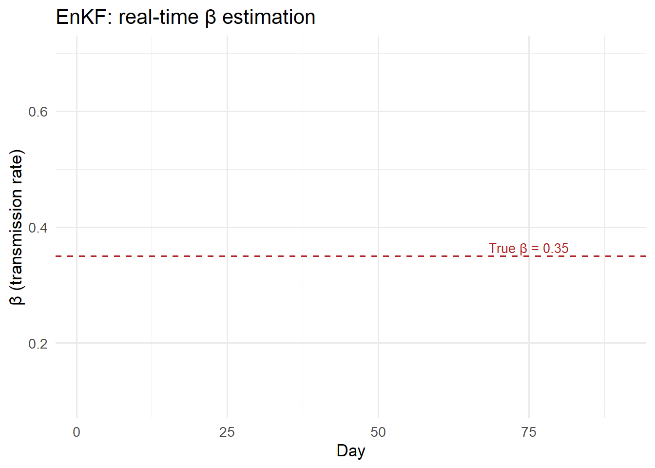
df_obs <- data.frame(
  day    = days_obs,
  median = fit$deltaI[, 1],
  lo     = fit$deltaI[, 2],
  hi     = fit$deltaI[, 3],
  obs    = obs
)

ggplot(df_obs, aes(x = day)) +
  geom_ribbon(aes(ymin = lo, ymax = hi), fill = "orange",
              alpha = 0.35) +
  geom_line(aes(y = median), colour = "darkorange", linewidth = 1) +
  geom_point(aes(y = obs), colour = "grey30", size = 0.9) +
  labs(x = "Day", y = "New cases",
       title = "One-step-ahead forecast vs observations") +
  theme_minimal(base_size = 13)
The filter recovers \(\beta\) close to its true value (0.35) after approximately 15 days of data, and the one-step-ahead forecasts track the observed counts closely throughout.
6 Key design choices
Ensemble size (\(N\)). Larger ensembles give better covariance estimates but are slower. For a 5-state problem, \(N = 200\)–\(500\) is usually sufficient. For high-dimensional spatial models, \(N\) may be \(10^3\)–\(10^4\).
Process noise on parameters. Adding a small random walk to \(\log \beta\) each step allows the filter to track slowly changing transmission rates (e.g., seasonality, behaviour change). The noise magnitude controls the speed of adaptation: too large causes jitter, too small prevents tracking.
Observation variance \(R\). We used obs[t] (Poisson-variance approximation). A better approach calibrates \(R\) from historical data or estimates it jointly.
Covariance inflation. If the ensemble collapses (all particles become similar), the filter can lose the ability to update. Multiplicative inflation — multiplying ensemble anomalies by a factor slightly greater than 1 — prevents this.
7 Connecting to a digital twin product
In a deployed system, the EnKF runs as a scheduled job (e.g., every night when new case counts are published):
New surveillance data
        │
        ▼
  Fetch from database  (Post 6: TimescaleDB)
        │
        ▼
  Run EnKF             (this post)
        │
        ▼
  Store posterior      (Post 6: TimescaleDB)
        │
        ▼
  Update dashboard     (Post 8: Streamlit)
The result is a model whose internal state continuously tracks reality — the defining property of an operational digital twin.
8 References
1.
Kalman RE. A new approach to linear filtering and prediction problems. Journal of Basic Engineering. 1960;82(1):35–45. doi:10.1115/1.3662552
2.
Evensen G. Sequential data assimilation with a nonlinear quasi-geostrophic model using Monte Carlo methods to forecast error statistics. Journal of Geophysical Research: Oceans. 1994;99(C5):10143–62. doi:10.1029/94JC00572
3.
Evensen G. The ensemble Kalman filter: Theoretical formulation and practical implementation. Ocean Dynamics. 2003;53:343–67. doi:10.1007/s10236-003-0036-9
4.
Shaman J, Karspeck A, Yang W, Tamerius J, Lipsitch M. Real-time influenza forecasts during the 2012–2013 season. Nature Communications. 2013;4:2837. doi:10.1038/ncomms3837