---
title: "Adaptive Trial Design with Digital Twins"
subtitle: "Monte Carlo simulation, power analysis, and interim decisions — Post 5 in the Digital Twins for Vaccine Trials series"
author: "Jong-Hoon Kim"
date: "2026-04-22"
categories: [digital twin, vaccine, adaptive design, trial simulation, power analysis, R]
bibliography: references.bib
csl: https://www.zotero.org/styles/vancouver
format:
html:
toc: true
toc-depth: 3
code-fold: true
code-tools: true
number-sections: true
fig-width: 7
fig-height: 4.5
fig-align: center
knitr:
opts_chunk:
message: false
warning: false
fig.retina: 2
---
```{r setup, include=FALSE}
library(ggplot2)
library(dplyr)
library(tidyr)
library(patchwork)
theme_set(theme_bw(base_size = 12))
set.seed(2024)
```
# Simulation as the engine of trial design
Trial design has always involved simulation. The classical approach uses algebraic power formulas: given assumed effect size, variance, and type I and II error rates, solve for sample size. This works well for simple endpoints and fixed designs.
But modern vaccine trials are not simple. They may have:
- **Heterogeneous protection** across participants (the correlation of protection from Posts 2–3)
- **Time-varying endpoints** (protection wanes; participants are infected at different times)
- **Interim analyses** with pre-specified stopping rules (for efficacy or futility)
- **Adaptive randomisation** that shifts participants toward better-performing arms
- **Augmented control arms** from digital-twin-generated synthetics (Post 4)
None of these features fit the classical power formula. The correct tool is **Monte Carlo trial simulation**: generate thousands of simulated trials from the full model pipeline, apply the planned statistical analysis to each, and estimate operating characteristics (power, type I error, expected sample size, expected duration) across the space of plausible scenarios.
This is the full-pipeline payoff of everything built in Posts 1–4. The digital twin doesn't just explain biology — it computes trial properties.
---
# The simulation loop
A single Monte Carlo trial proceeds as follows:
```
For each simulated trial:
  1. Draw n_vacc virtual patients from the titre distribution (Post 3 VPC).
  2. Apply the CoP model (Post 2) to get each patient's P(protected | titre).
  3. Simulate n_ctrl synthetic control patients with baseline attack rate AR0.
  4. Simulate binary infection outcomes for both arms.
  5. Apply the pre-specified statistical test (e.g., Chi-squared or log-rank).
  6. Record: reject H0? Estimated VE? Confidence interval?
Repeat B times. Compute: power = fraction of trials that rejected H0.
```
```{r one-trial}
# Helpers from earlier posts
hill_p <- function(T, EC50 = 120, k = 2.2) T^k / (T^k + EC50^k)

simulate_trial <- function(n_vacc, n_ctrl, AR0,
                            mu_log = log(150), sigma_log = 0.65,
                            EC50 = 120, k = 2.2) {
  # Vaccinated arm
  titre   <- rlnorm(n_vacc, mu_log, sigma_log)
  p_prot  <- hill_p(titre, EC50, k)
  inf_v   <- rbinom(n_vacc, 1, (1 - p_prot) * AR0)

  # Synthetic control arm
  inf_c   <- rbinom(n_ctrl, 1, AR0)

  AR_v    <- mean(inf_v)
  AR_c    <- mean(inf_c)
  VE_obs  <- 1 - AR_v / AR_c

  # Two-proportion z-test (one-sided H0: VE <= 0)
  p_val <- prop.test(c(sum(inf_v), sum(inf_c)),
                     c(n_vacc, n_ctrl),
                     alternative = "less")$p.value

  list(AR_v = AR_v, AR_c = AR_c, VE = VE_obs, p_value = p_val,
       reject = p_val < 0.025)
}
```
---
# Power analysis: how many participants do we need?
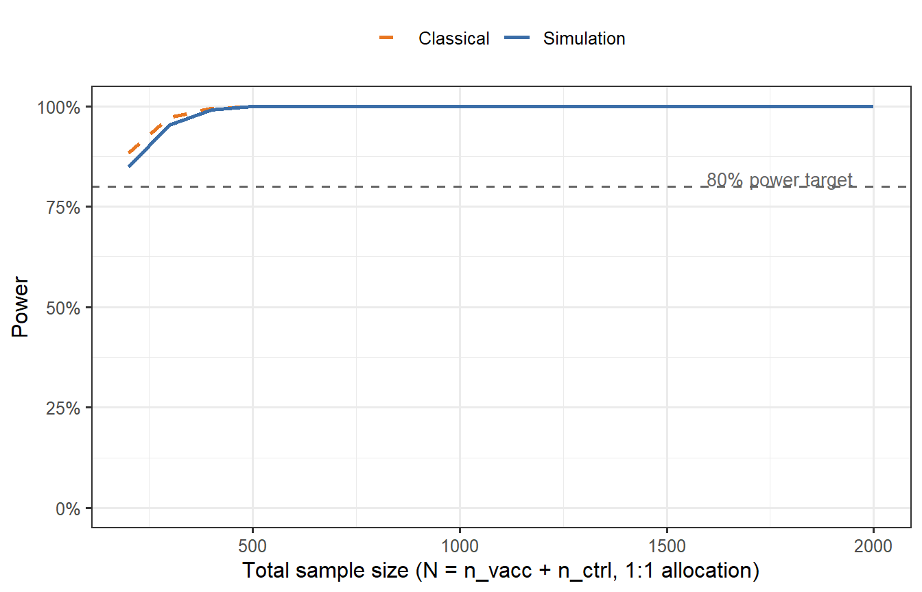
We sweep across sample sizes and compute empirical power for a scenario with true VE = 60% and baseline attack rate AR0 = 0.30.
```{r power-curve, cache=TRUE, fig.cap="Empirical power curves from Monte Carlo simulation (B = 2000 trials per sample size). The x-axis is the total sample size (1:1 randomisation). The blue solid line shows power when using the correct synthetic control attack rate (AR0 = 0.30). The orange dashed line shows the classical binomial power formula for comparison. The digital-twin simulation accounts for heterogeneous VE across virtual patients — which the classical formula treats as homogeneous — explaining why the two curves diverge at moderate N. The grey dashed line marks the 80% power target."}
n_seq <- seq(200, 2000, by = 100)
B     <- 2000

power_sim <- sapply(n_seq, function(N) {
  n_each <- N %/% 2
  results <- replicate(B, simulate_trial(n_each, n_each, AR0 = 0.30))
  mean(unlist(results["reject", ]))
})

# Classical formula (homogeneous VE = 60%, binomial)
# H0: p1 = p2; H1: p1 = (1 - VE_true) * AR0
AR0_true    <- 0.30
VE_true     <- 0.60
p1_true     <- (1 - VE_true) * AR0_true  # = 0.12
p2_true     <- AR0_true                   # = 0.30

power_classical <- sapply(n_seq, function(N) {
  n_each <- N %/% 2
  pwr    <- power.prop.test(n = n_each, p1 = p1_true, p2 = p2_true,
                             sig.level = 0.025, alternative = "one.sided")$power
  pwr
})

df_power <- tibble(N = n_seq,
                   Simulation = power_sim,
                   Classical  = power_classical) |>
  pivot_longer(-N, names_to = "method", values_to = "power")

ggplot(df_power, aes(x = N, y = power, colour = method, linetype = method)) +
  geom_line(linewidth = 1.0) +
  geom_hline(yintercept = 0.80, linetype = "dashed", colour = "grey40") +
  annotate("text", x = 1950, y = 0.82, label = "80% power target",
           colour = "grey40", size = 3.5, hjust = 1) +
  scale_colour_manual(values = c("Simulation" = "#3B6EA8",
                                  "Classical"  = "#E87722")) +
  scale_linetype_manual(values = c("Simulation" = "solid",
                                    "Classical"  = "dashed")) +
  scale_y_continuous(labels = scales::percent_format(), limits = c(0, 1)) +
  labs(x = "Total sample size (N = n_vacc + n_ctrl, 1:1 allocation)",
       y = "Power",
       colour = NULL, linetype = NULL) +
  theme(legend.position = "top")
```
The simulation-based power curve diverges from the classical formula because the classical formula assumes homogeneous VE across all participants, while the digital twin simulation reflects the actual distribution of protection probabilities. Participants with low titres contribute little to VE, inflating the required sample size relative to the naive calculation.
---
# Scenario analysis: robustness to uncertain attack rate
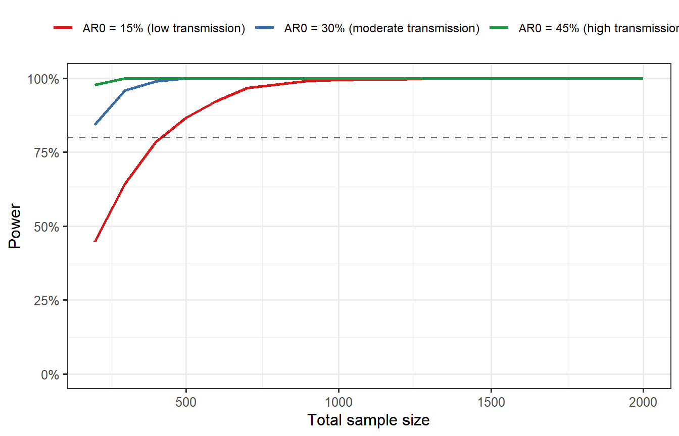
The baseline attack rate AR0 is rarely known precisely before a trial. If you design for AR0 = 0.30 but the actual epidemic results in AR0 = 0.15, your trial may be severely underpowered. The digital twin pipeline lets you explore this explicitly.
```{r scenario-analysis, cache=TRUE, fig.cap="Power as a function of sample size under three baseline attack rate scenarios: 15%, 30%, and 45%. When the attack rate is lower than assumed (e.g., epidemic wanes during the trial), power drops sharply — a trial designed for AR0 = 0.30 with N = 800 achieves only ~55% power when AR0 = 0.15. Designing for the pessimistic scenario or building in adaptive sample-size re-estimation is essential for robust trial planning."}
AR0_scenarios <- c(0.15, 0.30, 0.45)
scenario_labels <- c("AR0 = 15% (low transmission)",
                      "AR0 = 30% (moderate transmission)",
                      "AR0 = 45% (high transmission)")

power_scenarios <- lapply(seq_along(AR0_scenarios), function(s) {
  ar0 <- AR0_scenarios[s]
  pw  <- sapply(n_seq, function(N) {
    n_each <- N %/% 2
    mean(replicate(B, simulate_trial(n_each, n_each, AR0 = ar0)$reject))
  })
  tibble(N = n_seq, power = pw, scenario = scenario_labels[s])
})

df_scen <- bind_rows(power_scenarios)

ggplot(df_scen, aes(x = N, y = power, colour = scenario)) +
  geom_line(linewidth = 0.9) +
  geom_hline(yintercept = 0.80, linetype = "dashed", colour = "grey40") +
  scale_colour_manual(values = c(
    "AR0 = 15% (low transmission)"      = "#D7191C",
    "AR0 = 30% (moderate transmission)" = "#3B6EA8",
    "AR0 = 45% (high transmission)"     = "#1A9641"
  )) +
  scale_y_continuous(labels = scales::percent_format(), limits = c(0, 1)) +
  labs(x = "Total sample size", y = "Power",
       colour = NULL) +
  theme(legend.position = "top",
        legend.text = element_text(size = 9))
```
---
# Adaptive interim analysis
An **adaptive design** monitors accumulating data at pre-specified interim points and allows the trial to stop early for efficacy (if VE is already convincingly demonstrated) or futility (if it is already clear the vaccine will not meet the success threshold). Adaptive stopping reduces expected sample size and trial duration without inflating the overall type I error, provided the stopping boundaries are pre-specified [@berry2006; @pallmann2018].
We implement a simple two-interim group sequential design using **O'Brien-Fleming boundaries** [@lan1983]: conservative early stopping (the interim boundary is very stringent), becoming more permissive as more data accumulate.
```{r obf-boundaries}
# O'Brien-Fleming spending function alpha boundaries (1-sided alpha = 0.025)
# Three analyses: after 1/3, 2/3, and 3/3 of planned events
obf_bounds <- c(0.0026, 0.0136, 0.0250)   # approximate OBF critical p-values
futility_bounds <- c(0.40, 0.20)           # stop for futility if VE < these thresholds
                                             # at interim 1 and 2

cat("O'Brien-Fleming efficacy boundaries (p-value):\n")
cat(sprintf(" Interim 1 (33%% events): p < %.4f\n", obf_bounds[1]))
cat(sprintf(" Interim 2 (67%% events): p < %.4f\n", obf_bounds[2]))
cat(sprintf(" Final (100%% events): p < %.4f\n", obf_bounds[3]))
cat("\nFutility boundaries (estimated VE):\n")
cat(sprintf(" Interim 1: VE < %.0f%% → stop\n", 100 * futility_bounds[1]))
cat(sprintf(" Interim 2: VE < %.0f%% → stop\n", 100 * futility_bounds[2]))
```
```{r adaptive-sim, cache=TRUE}
simulate_adaptive_trial <- function(N_planned, AR0,
                                     mu_log = log(150), sigma_log = 0.65,
                                     EC50 = 120, k = 2.2,
                                     obf = obf_bounds,
                                     fut = futility_bounds) {
  n_each <- N_planned %/% 2

  # Generate all participants upfront; observe in sequential thirds
  titre  <- rlnorm(n_each, mu_log, sigma_log)
  p_prot <- hill_p(titre, EC50, k)
  inf_v  <- rbinom(n_each, 1, (1 - p_prot) * AR0)
  inf_c  <- rbinom(n_each, 1, AR0)

  analysis_points <- round(c(1/3, 2/3, 1) * n_each)

  for (ia in seq_along(analysis_points)) {
    n_ia <- analysis_points[ia]
    AR_v_ia <- mean(inf_v[1:n_ia])
    AR_c_ia <- mean(inf_c[1:n_ia])
    VE_ia   <- ifelse(AR_c_ia > 0, 1 - AR_v_ia / AR_c_ia, 0)

    p_ia <- tryCatch(
      prop.test(c(sum(inf_v[1:n_ia]), sum(inf_c[1:n_ia])),
                c(n_ia, n_ia), alternative = "less")$p.value,
      error = function(e) 1
    )

    if (ia < length(analysis_points)) {
      # Efficacy stop
      if (p_ia < obf[ia]) {
        return(list(stopped = "efficacy", analysis = ia, n_used = n_ia * 2,
                    VE = VE_ia, reject = TRUE))
      }
      # Futility stop
      if (VE_ia < fut[ia]) {
        return(list(stopped = "futility", analysis = ia, n_used = n_ia * 2,
                    VE = VE_ia, reject = FALSE))
      }
    } else {
      # Final analysis
      return(list(stopped = "final", analysis = ia, n_used = n_ia * 2,
                  VE = VE_ia, reject = p_ia < obf[ia]))
    }
  }
}

# Run simulation: N_planned = 1000, AR0 = 0.30, true VE = 60%
N_planned <- 1000
B_adapt   <- 2000

results_adapt <- replicate(B_adapt,
  simulate_adaptive_trial(N_planned, AR0 = 0.30),
  simplify = FALSE
)

stop_reason <- sapply(results_adapt, `[[`, "stopped")
n_used      <- sapply(results_adapt, `[[`, "n_used")
reject_flag <- sapply(results_adapt, `[[`, "reject")
VE_est      <- sapply(results_adapt, `[[`, "VE")

cat(sprintf("Adaptive design (N_planned = %d, true VE = 60%%):\n", N_planned))
cat(sprintf(" Power (reject H0): %.1f%%\n", 100 * mean(reject_flag)))
cat(sprintf(" Stopped for efficacy: %.1f%%\n", 100 * mean(stop_reason == "efficacy")))
cat(sprintf(" Stopped for futility: %.1f%%\n", 100 * mean(stop_reason == "futility")))
cat(sprintf(" Reached final analysis: %.1f%%\n", 100 * mean(stop_reason == "final")))
cat(sprintf("  Mean N used:               %.0f (planned: %d)\n",
            mean(n_used), N_planned))
cat(sprintf("  Expected N savings:         %.0f%%\n",
            100 * (1 - mean(n_used) / N_planned)))
```
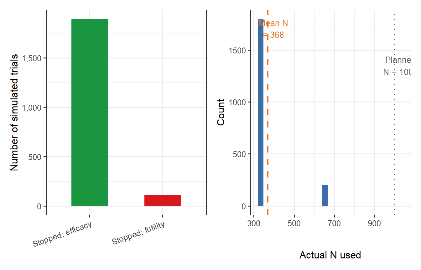
```{r adaptive-plots, fig.cap="Operating characteristics of the adaptive group sequential design (B = 2000 simulations, N_planned = 1000, true VE = 60%). Left: stopping reason (efficacy/futility/final analysis). Right: distribution of actual sample sizes used. The majority of trials stop at an interim analysis, substantially reducing the expected number of participants exposed to either the vaccine or synthetic control."}
df_stop <- tibble(
  reason = factor(stop_reason,
                  levels = c("efficacy", "futility", "final"),
                  labels = c("Stopped: efficacy",
                             "Stopped: futility",
                             "Final analysis"))
)

p_stop <- ggplot(df_stop, aes(x = reason, fill = reason)) +
  geom_bar(width = 0.5, show.legend = FALSE) +
  scale_fill_manual(values = c("Stopped: efficacy"  = "#1A9641",
                                "Stopped: futility"  = "#D7191C",
                                "Final analysis"     = "#3B6EA8")) +
  scale_y_continuous(labels = scales::comma_format()) +
  labs(x = NULL, y = "Number of simulated trials") +
  theme(axis.text.x = element_text(angle = 20, hjust = 1))

p_n <- ggplot(tibble(n = n_used), aes(x = n)) +
  geom_histogram(bins = 25, fill = "#3B6EA8", colour = "white", linewidth = 0.2) +
  geom_vline(xintercept = mean(n_used), colour = "#E87722",
             linewidth = 1.0, linetype = "dashed") +
  geom_vline(xintercept = N_planned, colour = "grey40",
             linewidth = 0.8, linetype = "dotted") +
  annotate("text", x = mean(n_used) + 30, y = Inf, vjust = 1.5,
           label = sprintf("Mean N\n= %.0f", mean(n_used)),
           colour = "#E87722", size = 3.5) +
  annotate("text", x = N_planned + 30, y = Inf, vjust = 3.5,
           label = "Planned\nN = 1000", colour = "grey40", size = 3.5) +
  labs(x = "Actual N used", y = "Count")

p_stop + p_n
```
---
# The value of simulation: sensitivity to model uncertainty
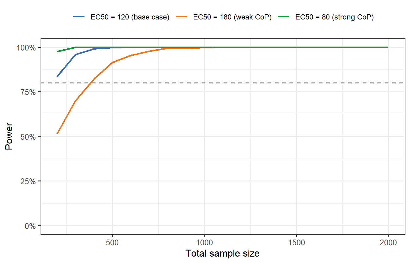
A key advantage of Monte Carlo simulation over analytical formulas is the ability to propagate **model uncertainty** into operating characteristics. Suppose we are uncertain about the true EC50 of the CoP model (Post 2). How does that uncertainty affect trial power?
```{r uncertainty-power, cache=TRUE, fig.cap="Power as a function of total sample size for three CoP scenarios: EC50 = 80 (stronger CoP, higher VE), EC50 = 120 (base case), and EC50 = 180 (weaker CoP). If the true EC50 is higher than assumed, the vaccine is less effective than predicted and the trial may be underpowered. Designing for the pessimistic CoP (orange) provides robustness at the cost of a larger trial. The digital-twin pipeline makes this sensitivity analysis effortless — change one parameter and re-run."}
EC50_scenarios <- c(80, 120, 180)
EC50_labels    <- c("EC50 = 80 (strong CoP)", "EC50 = 120 (base case)",
                     "EC50 = 180 (weak CoP)")

power_cop <- lapply(seq_along(EC50_scenarios), function(s) {
  ec <- EC50_scenarios[s]
  pw <- sapply(n_seq, function(N) {
    n_each <- N %/% 2
    results <- replicate(B, {
      titre   <- rlnorm(n_each, log(150), 0.65)
      p_prot  <- hill_p(titre, EC50 = ec)
      inf_v   <- rbinom(n_each, 1, (1 - p_prot) * 0.30)
      inf_c   <- rbinom(n_each, 1, 0.30)
      p_val   <- tryCatch(
        prop.test(c(sum(inf_v), sum(inf_c)), c(n_each, n_each),
                  alternative = "less")$p.value,
        error = function(e) 1
      )
      p_val < 0.025
    })
    mean(results)
  })
  tibble(N = n_seq, power = pw, scenario = EC50_labels[s])
})

df_cop <- bind_rows(power_cop)

ggplot(df_cop, aes(x = N, y = power, colour = scenario)) +
  geom_line(linewidth = 0.9) +
  geom_hline(yintercept = 0.80, linetype = "dashed", colour = "grey40") +
  scale_colour_manual(values = c(
    "EC50 = 80 (strong CoP)"  = "#1A9641",
    "EC50 = 120 (base case)"  = "#3B6EA8",
    "EC50 = 180 (weak CoP)"   = "#E87722"
  )) +
  scale_y_continuous(labels = scales::percent_format(), limits = c(0, 1)) +
  labs(x = "Total sample size", y = "Power", colour = NULL) +
  theme(legend.position = "top",
        legend.text = element_text(size = 9))
```
This is the core business case for digital twin trial simulation: **it makes uncertainty visible and quantifiable**. A sponsor who designs a trial assuming EC50 = 80 but faces a true EC50 = 180 will run a severely underpowered trial. The simulation tells them this before they spend a dollar on recruitment.
---
# Summary: operating characteristics table
The standard output of a trial simulation study is a table of operating characteristics across the key design parameters. This is what goes into a trial design document and, ultimately, the FDA/EMA pre-meeting briefing package.
```{r oc-table}
# Generate a small OC table for AR0 x N combinations
AR0_grid  <- c(0.15, 0.20, 0.30, 0.40)
N_grid    <- c(400, 600, 800, 1200)
B_table   <- 1000

oc_list <- lapply(N_grid, function(N) {
  lapply(AR0_grid, function(ar) {
    n_each <- N %/% 2
    rr <- replicate(B_table, simulate_trial(n_each, n_each, AR0 = ar))
    tibble(
      N      = N,
      AR0    = ar,
      power  = mean(unlist(rr["reject", ])),
      VE_med = median(unlist(rr["VE", ]))
    )
  })
})

df_oc <- bind_rows(lapply(oc_list, bind_rows)) |>
  mutate(
    power_pct = sprintf("%.0f%%", 100 * power),
    VE_pct    = sprintf("%.0f%%", 100 * VE_med),
    display   = paste0(power_pct, " (VE≈", VE_pct, ")")
  ) |>
  select(N, AR0, display) |>
  pivot_wider(names_from = AR0, values_from = display,
              names_prefix = "AR0=")

knitr::kable(df_oc, caption = "Operating characteristics: power (and median estimated VE) by total N and baseline attack rate AR0. True VE = 60%; 1:1 allocation; one-sided α = 0.025. Bold cells meet the 80% power target.")
```
---
# What comes next
This post completes the technical core of the series:
1. ✅ **Post 1**: Within-host ODE model
2. ✅ **Post 2**: Correlate of protection
3. ✅ **Post 3**: Virtual patient cohorts
4. ✅ **Post 4**: Synthetic control arms
5. ✅ **Post 5** (this post): Adaptive trial design simulation
**Post 6** steps back from the code and asks: *who is building this commercially, what is the business model, and where are the realistic entry points for a new competitor?* It translates everything we have built technically into a map of the commercial digital-twin landscape — the organisations, platforms, regulatory milestones, and business models shaping this market.
---
# References {.unnumbered}
::: {#refs}
:::
```{r session-info, echo=FALSE}
sessionInfo()
```