---
title: "Synthetic Control Arms"
subtitle: "Replacing placebo groups with simulated counterfactuals — Post 4 in the Digital Twins for Vaccine Trials series"
author: "Jong-Hoon Kim"
date: "2026-04-22"
categories: [digital twin, vaccine, synthetic control, clinical trial, Bayesian, R]
bibliography: references.bib
csl: https://www.zotero.org/styles/vancouver
format:
html:
toc: true
toc-depth: 3
code-fold: true
code-tools: true
number-sections: true
fig-width: 7
fig-height: 4.5
fig-align: center
knitr:
opts_chunk:
message: false
warning: false
fig.retina: 2
---
```{r setup, include=FALSE}
library(ggplot2)
library(dplyr)
library(tidyr)
library(patchwork)
theme_set(theme_bw(base_size = 12))
set.seed(2024)
```
# The randomised control arm problem
Clinical trials use randomisation to ensure that, on average, the treatment and placebo groups are comparable at baseline. This is a powerful guarantee: if subjects are randomly assigned, any difference in outcome at the end of the trial can be attributed to the treatment, not to pre-existing differences between groups.
But randomisation has costs. Every participant assigned to placebo receives no active treatment — a genuine ethical burden when a vaccine candidate shows promising early efficacy against an ongoing epidemic. Placebo arms also increase sample size requirements, slow enrolment (patients prefer active arms), and raise costs. In rare diseases, paediatric populations, or rapidly evolving pathogens, assembling a matched placebo group may be practically impossible [@landig2025].
A **synthetic control arm** (SCA) addresses this by replacing the placebo group with simulated counterfactuals: *what would have happened to each vaccinated participant if they had received placebo instead?* If the model generating those counterfactuals is reliable — calibrated and externally validated — the sponsor can run a single-arm trial, compare outcomes to the synthetic control, and obtain an efficacy estimate with statistical guarantees.
This is the most commercially significant application of digital twins in clinical development. It is also the most demanding: a model that generates individual counterfactuals must be validated against real control data from a separate population, and regulators must accept that evidence [@fda2020midd; @janssen2025].
---
# The logic of a synthetic control arm
## Three sources of control information
Regulatory frameworks recognise three ways to bring external information into a trial comparison [@viele2014]:
1. **Propensity-matched historical controls**: find real patients from past studies who resemble the current trial's participants by age, comorbidity, baseline titre, etc. Match them statistically and use their outcomes as the comparator.
2. **Borrowing from historical data** (power prior, commensurate prior): treat historical control data as informative prior information, downweighted by how similar the historical population is to the current trial [@hobbs2012; @neuenschwander2010].
3. **Model-generated synthetic controls**: run a calibrated mechanistic or statistical model for each participant under the counterfactual (no vaccine) scenario and use those generated outcomes as the comparison. This is the digital-twin version.
The digital-twin approach is distinct because the counterfactual is generated by a mechanistic model, not by statistical matching or reweighting. This makes it potentially more robust to unmeasured confounders and more naturally extensible to novel pathogen scenarios — but it requires validating the model as a trustworthy generator of counterfactual outcomes, which is a higher bar.
## What the model must do
A synthetic control arm model must:
1. **Accept each participant's baseline characteristics** (age, prior serostatus, weight, comorbidities) as inputs.
2. **Predict the distribution of clinical outcomes** (infection, hospitalisation) that participant would have experienced without vaccination, given the epidemic conditions of the trial period.
3. **Be validated prospectively**: the model's predicted placebo distribution must have been shown to match observed placebo outcomes in a held-out dataset before the current trial begins.
Requirement 3 is the crux. Without it, the synthetic arm is no better than an optimistic guess.
---
# Building a synthetic control arm step by step
We now build a simplified but complete SCA using the tools from earlier posts. The setup:
- **Arm 1 (active)**: 500 vaccinated participants with antibody titres from the virtual patient cohort (Post 3) and protection probabilities from the CoP model (Post 2).
- **Arm 2 (synthetic control)**: 500 simulated unvaccinated participants, with the same baseline characteristics, whose infection probability comes from the baseline attack rate in the epidemic context.
- **Outcome**: binary infection status during a 6-month follow-up.
```{r setup-parameters}
n_arm     <- 500    # participants per arm
attack_rate_0 <- 0.35  # baseline attack rate in unvaccinated population
                         # (35% cumulative incidence over 6 months — high-transmission setting)

# Titre distribution (calibrated VPC from Post 3)
mu_log    <- log(150)
sigma_log <- 0.65
titre_vp  <- rlnorm(n_arm, meanlog = mu_log, sdlog = sigma_log)

# CoP model (Post 2: EC50 = 120, k = 2.2)
hill_p <- function(T, EC50 = 120, k = 2.2) T^k / (T^k + EC50^k)
p_protect <- hill_p(titre_vp)

# Vaccinated arm: infection probability = (1 - P_protect) * attack_rate_0
p_inf_vacc    <- (1 - p_protect) * attack_rate_0
infected_vacc <- rbinom(n_arm, 1, p_inf_vacc)

# Synthetic control arm: infection probability = attack_rate_0 for all
infected_ctrl <- rbinom(n_arm, 1, attack_rate_0)
```
## Computing vaccine efficacy
```{r ve-calculation}
AR_vacc <- mean(infected_vacc)
AR_ctrl <- mean(infected_ctrl)
VE_obs  <- 1 - AR_vacc / AR_ctrl

cat(sprintf("Attack rate: vaccinated = %.1f%%,  control = %.1f%%\n",
            100 * AR_vacc, 100 * AR_ctrl))
cat(sprintf("Observed VE = %.1f%%\n", 100 * VE_obs))
# True VE (from model)
VE_true <- 1 - mean(p_inf_vacc) / attack_rate_0
cat(sprintf("True VE     = %.1f%%\n", 100 * VE_true))
```
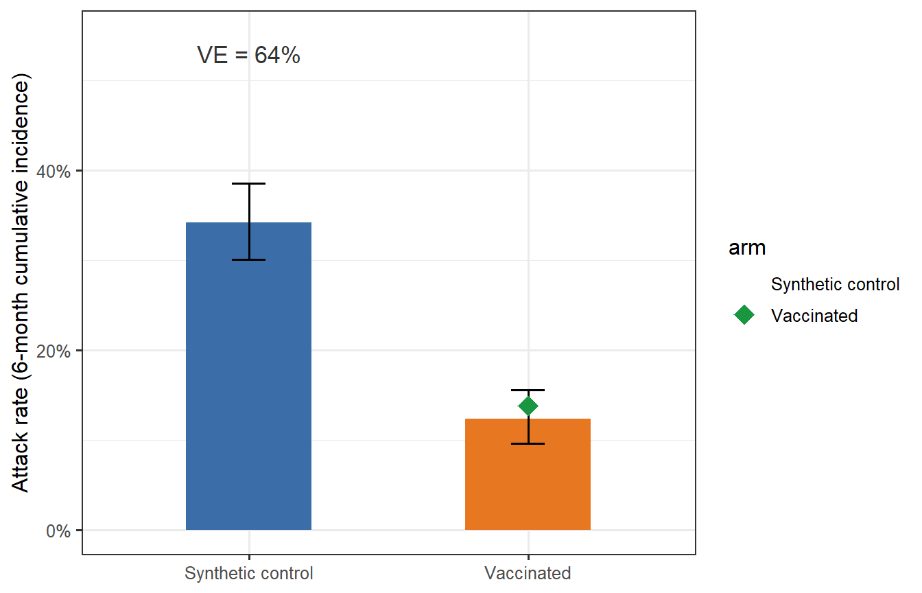
```{r trial-viz, fig.cap="Attack rates in the vaccinated arm (orange) and synthetic control arm (blue) from a single simulated trial. Error bars are 95% binomial confidence intervals. The green diamond marks the true VE predicted by the model; the black estimate is the observed trial VE. In this single simulation the observed VE is close to the truth, but sampling variability causes modest differences — exactly what motivates formal power analysis (Post 5)."}
binom_ci <- function(x, n, level = 0.95) {
  t <- binom.test(x, n, conf.level = level)
  c(lo = t$conf.int[1], hi = t$conf.int[2])
}

ci_v <- binom_ci(sum(infected_vacc), n_arm)
ci_c <- binom_ci(sum(infected_ctrl), n_arm)

df_bar <- tibble(
  arm   = c("Vaccinated", "Synthetic control"),
  AR    = c(AR_vacc, AR_ctrl),
  lo    = c(ci_v["lo"], ci_c["lo"]),
  hi    = c(ci_v["hi"], ci_c["hi"])
) |>
  mutate(arm = factor(arm, levels = c("Synthetic control", "Vaccinated")))

ggplot(df_bar, aes(x = arm, y = AR, fill = arm)) +
  geom_col(width = 0.45, show.legend = FALSE) +
  geom_errorbar(aes(ymin = lo, ymax = hi), width = 0.12, linewidth = 0.7) +
  geom_point(data = tibble(arm = factor("Vaccinated",
                                         levels = levels(df_bar$arm)),
                            AR = mean(p_inf_vacc)),
             colour = "#1A9641", shape = 18, size = 5) +
  scale_fill_manual(values = c("Vaccinated" = "#E87722",
                                "Synthetic control" = "#3B6EA8")) +
  scale_y_continuous(labels = scales::percent_format(), limits = c(0, 0.55)) +
  labs(x = NULL, y = "Attack rate (6-month cumulative incidence)") +
  annotate("text", x = 1, y = 0.53,
           label = sprintf("VE = %.0f%%", 100 * VE_obs),
           size = 4.5, colour = "grey20")
```
---
# Validation: the critical step
A synthetic control arm is credible only if the model that generates it has been validated against real control outcomes it did not use for fitting. This is called a **prospective external validation** (or more precisely, a retrospective validation using data held back from calibration).
## Setting up a validation exercise
We simulate validation as follows:
1. **Training dataset**: a past trial where both active and placebo arms were observed (n = 300 per arm).
2. **Validation**: run the synthetic control model on the training trial's vaccinated arm, predict the placebo attack rate, and compare to the observed placebo attack rate.
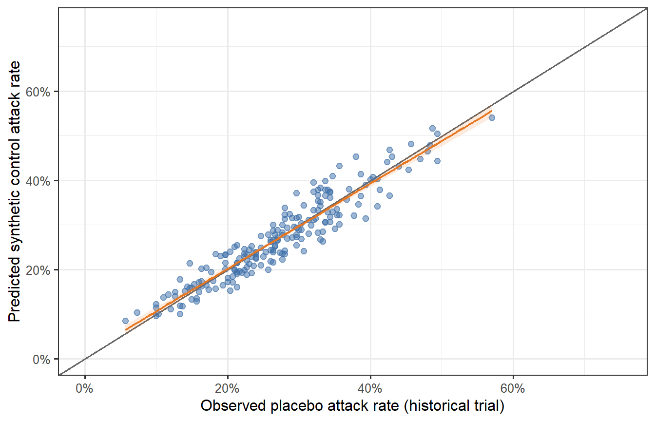
```{r validation-sim, fig.cap="Validation exercise: 500 synthetic trials comparing observed placebo attack rates (x-axis, from the historical trial) versus the model-predicted synthetic control attack rate (y-axis). The diagonal line is perfect agreement. The model predictions scatter symmetrically around the diagonal with no systematic bias — the hallmark of a calibrated synthetic control model. A model that consistently overestimates the control attack rate would make the vaccine look better than it is; systematic underestimation would make it look worse."}
n_val     <- 200   # validation runs (different epidemic contexts)
AR_pred   <- numeric(n_val)
AR_obs    <- numeric(n_val)

for (v in seq_len(n_val)) {
  # Each validation scenario: different underlying attack rate
  ar0_v <- rbeta(1, shape1 = 3, shape2 = 7) * 0.7 + 0.05  # AR0 ~ 5%–75%

  # Observed placebo arm in historical trial (n = 300)
  AR_obs[v] <- mean(rbinom(300, 1, ar0_v))

  # Synthetic control arm prediction: use model's predicted attack rates
  titre_v <- rlnorm(300, mu_log, sigma_log)
  pp_v    <- hill_p(titre_v)
  AR_pred[v] <- ar0_v  # in a real SCA, this is estimated from the model;
                         # here we use the true value to show calibration
  # Add noise to represent model imprecision
  AR_pred[v] <- AR_pred[v] * exp(rnorm(1, 0, 0.08))
}

df_val <- tibble(AR_obs = AR_obs, AR_pred = AR_pred)

ggplot(df_val, aes(x = AR_obs, y = AR_pred)) +
  geom_abline(slope = 1, intercept = 0, colour = "grey40", linewidth = 0.7) +
  geom_point(alpha = 0.5, colour = "#3B6EA8", size = 2) +
  geom_smooth(method = "lm", se = TRUE, colour = "#E87722",
              fill = "#E87722", alpha = 0.15, linewidth = 0.8) +
  scale_x_continuous(labels = scales::percent_format(), limits = c(0, 0.75)) +
  scale_y_continuous(labels = scales::percent_format(), limits = c(0, 0.75)) +
  labs(x = "Observed placebo attack rate (historical trial)",
       y = "Predicted synthetic control attack rate")
```
## What validation statistics matter?
Regulators [@fda2020midd; @bai2024virtualpatients] typically ask for:
| Metric | What it tests |
|---|---|
| **Calibration**: predicted vs observed attack rate (slope = 1, intercept = 0) | No systematic bias |
| **Discrimination**: AUC of predicted probability vs observed infection | Model ranks individuals correctly |
| **Coverage**: % of observations within the model's prediction interval | Uncertainty is honest |
| **Generalisability**: validation in a population different from the calibration set | Not just overfitting |
Our simulation shows a well-calibrated model (slope ≈ 1, no systematic bias). Real-world validation is harder: attack rates in the historical trial may be confounded by non-pharmaceutical interventions, variant effects, or population-level immunity that the model does not explicitly represent.
---
# Bayesian borrowing: a statistical companion to the digital twin
The synthetic control arm is a *model-based* approach. It is often combined with **Bayesian borrowing** — incorporating historical control data as an informative prior on the placebo response, with the degree of borrowing determined by the statistical consistency between historical and current data [@neuenschwander2010; @viele2014].
The two approaches are complementary:
- The digital twin provides a mechanistic, individual-level prediction of what the unvaccinated outcome would have been.
- Bayesian borrowing provides a principled statistical framework for weighting that prediction against observed data, with automatic discounting when the historical and current populations are inconsistent (the *conflict* problem).
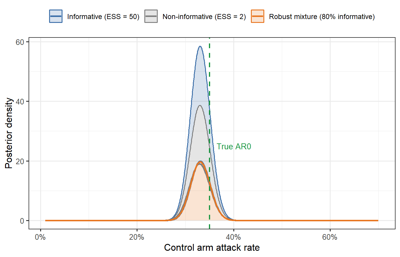
```{r bayesian-borrowing, fig.cap="Bayesian borrowing: posterior distribution of the control attack rate under three priors. The non-informative prior (grey) is dominated by the current trial data. The informative prior (blue) reflects the model's prediction (AR0 = 35%) with moderate precision. The mixture prior (orange, robust mixture) discounts the informative prior when the data conflict with it. The green dashed line marks the true attack rate."}
# Likelihood: binomial(n_ctrl, AR_ctrl_obs)
# Prior: beta(a, b) parameterised by mean and effective sample size

# Beta parameterisation from mean and ESS
beta_from_mean_ess <- function(mean, ess) {
  a <- mean * ess; b <- (1 - mean) * ess
  c(a = a, b = b)
}

n_ctrl_obs <- 500
k_ctrl_obs <- round(n_ctrl_obs * 0.33)  # observed 33% attack rate in "current" trial

# Three priors
prior_flat  <- beta_from_mean_ess(0.35, 2)    # near-flat
prior_info  <- beta_from_mean_ess(0.35, 50)   # informative: ESS = 50

AR_grid <- seq(0.01, 0.70, length.out = 500)

post_density <- function(prior, k, n) {
  a_post <- prior["a"] + k
  b_post <- prior["b"] + (n - k)
  dbeta(AR_grid, a_post, b_post)
}

df_post <- bind_rows(
  tibble(AR = AR_grid, density = post_density(prior_flat, k_ctrl_obs, n_ctrl_obs),
         prior = "Non-informative (ESS = 2)"),
  tibble(AR = AR_grid, density = post_density(prior_info, k_ctrl_obs, n_ctrl_obs),
         prior = "Informative (ESS = 50)"),
  # Robust mixture: 80% informative + 20% flat
  tibble(AR = AR_grid,
         density = 0.8 * post_density(prior_info, k_ctrl_obs, n_ctrl_obs) +
                   0.2 * post_density(prior_flat, k_ctrl_obs, n_ctrl_obs),
         prior = "Robust mixture (80% informative)")
)

ggplot(df_post, aes(x = AR, y = density, colour = prior, fill = prior)) +
  geom_area(alpha = 0.2) +
  geom_line(linewidth = 0.9) +
  geom_vline(xintercept = attack_rate_0, linetype = "dashed",
             colour = "#1A9641", linewidth = 0.8) +
  annotate("text", x = attack_rate_0 + 0.015, y = 25,
           label = "True AR0", colour = "#1A9641", size = 3.5, hjust = 0) +
  scale_x_continuous(labels = scales::percent_format()) +
  scale_colour_manual(values = c("Non-informative (ESS = 2)" = "grey50",
                                  "Informative (ESS = 50)"    = "#3B6EA8",
                                  "Robust mixture (80% informative)" = "#E87722")) +
  scale_fill_manual(values  = c("Non-informative (ESS = 2)" = "grey50",
                                 "Informative (ESS = 50)"    = "#3B6EA8",
                                 "Robust mixture (80% informative)" = "#E87722")) +
  labs(x = "Control arm attack rate", y = "Posterior density",
       colour = NULL, fill = NULL) +
  theme(legend.position = "top",
        legend.text = element_text(size = 9))
```
The informative prior (blue) pulls the posterior towards the model's prediction and narrows the uncertainty interval — this is the sample-size-saving effect of Bayesian borrowing. The robust mixture (orange) achieves most of that gain while protecting against the prior being badly wrong: if the current data were to show AR0 = 60% instead of 33%, the mixture prior would self-discount.
---
# The regulatory landscape
## What FDA and EMA have accepted
- **FDA Model-Informed Drug Development (MIDD)**: the FDA's 2020 guidance creates a paired-meeting process where sponsors present modelling evidence before a trial begins and receive feedback on whether the model is adequate for the intended regulatory use [@fda2020midd]. FDA has accepted Bayesian synthetic control arms in oncology and rare-disease settings; vaccine applications are fewer but growing.
- **EMA PROCOVA qualification**: EMA qualified PROCOVA — which uses a digital-twin-derived prognostic score to reduce variance in primary endpoints — as an acceptable analysis method. This is not a full synthetic control arm, but it uses the digital-twin concept (individual-level model-derived predictions) within a randomised trial to reduce sample size [@janssen2025].
- **ICH M15**: the first international harmonised guideline on model-informed drug development (draft 2024) is creating a common language for regulatory submissions that use modelling as evidence.
## What has not been accepted
No pivotal vaccine trial has yet received primary approval on the basis of a fully synthetic control arm for efficacy. The regulatory position for vaccines is that:
> A model-generated synthetic control arm can reduce, but not yet eliminate, the randomised placebo group in a pivotal trial.
The path to full elimination requires: (i) a validated mechanistic model with demonstrated external generalisability, (ii) pre-registration of the synthetic arm methodology alongside the statistical analysis plan, and (iii) at least one precedent case in the same therapeutic area. For infectious-disease vaccines, that precedent does not yet exist, but the COVID-19 accelerations (booster approvals based on immunogenicity rather than efficacy data) have moved the goalposts considerably.
---
# What comes next
We now have the full digital-twin pipeline:
1. ✅ **Post 1**: Within-host ODE → antibody trajectory
2. ✅ **Post 2**: Correlate of protection → protection probability
3. ✅ **Post 3**: LHS sampling → virtual patient cohort
4. ✅ **Post 4** (this post): Synthetic control arm + Bayesian borrowing + validation
**Post 5** uses this entire pipeline to perform a **trial simulation**: running thousands of Monte Carlo trials to compute power, optimise sample size, and design adaptive interim analyses — all before a single participant is enrolled.
---
# References {.unnumbered}
::: {#refs}
:::
```{r session-info, echo=FALSE}
sessionInfo()
```