---
title: "Muscle Digital Twins: Science, Opportunity, and Directions"
subtitle: "Modelling individual adaptation to resistance training — and why it matters beyond the gym"
author: "Jong-Hoon Kim"
date: "2026-04-22"
categories: [digital twin, muscle, ODE, R, sarcopenia, business]
bibliography: references.bib
csl: https://www.zotero.org/styles/vancouver
format:
html:
toc: true
toc-depth: 3
code-fold: true
code-tools: true
number-sections: true
fig-width: 7
fig-height: 4.5
fig-align: center
knitr:
opts_chunk:
message: false
warning: false
fig.retina: 2
---
```{r setup, include=FALSE}
library(deSolve)
library(ggplot2)
library(dplyr)
library(tidyr)
library(patchwork)
```
# Why muscle?
Skeletal muscle is one of the most tractable organs for digital-twin modelling.
Its adaptation to mechanical loading follows dose–response kinetics that can be
written down as differential equations, measured non-invasively (force output,
muscle cross-sectional area by ultrasound, circulating biomarkers), and validated
against observable endpoints on timescales of weeks.
Muscle mass is also a frontline public health variable. Sarcopenia — the
age-related loss of muscle mass and function — affects an estimated 10–30% of
adults over 60 and is independently associated with falls, fractures,
hospitalisation, and all-cause mortality [@cruzjentoft2019]. The trajectory
toward sarcopenia begins silently in the fourth decade; a calibrated individual
model that predicts the trajectory and identifies optimal intervention timing has
direct clinical value.
This post builds a three-layer computational model in R, assesses the business
landscape honestly, and proposes directions where mechanistic modelling adds the
most value over current practice.
---
# The biology in brief
## Molecular stimulus: mTOR and protein turnover
Resistance exercise induces mechanical strain in muscle fibres, activating a
signalling cascade centred on the mechanistic target of rapamycin complex 1
(mTORC1) [@bodine2001]. mTORC1 phosphorylates p70S6K and 4E-BP1, accelerating
ribosomal translation of structural proteins — a process called *muscle protein
synthesis* (MPS). Simultaneously, protein degradation (MPB) continues at a
baseline rate. Net hypertrophy occurs when MPS exceeds MPB:
$$
\frac{dM}{dt} = k_s \cdot S(t) \cdot N(t) - k_d \cdot M
$$
where $M$ is muscle mass (kg), $S(t)$ is the mechanical training stimulus
(proportional to load × volume), $N(t)$ is a nutritional adequacy coefficient
(leucine availability is the key proximal signal), and $k_s$, $k_d$ are synthesis
and degradation rate constants. This equation is a simplification of a much
richer biochemical network, but it is sufficient to generate the qualitative
behaviours needed for a trial-design or clinical-monitoring digital twin.
## Macroscopic performance: the fitness–fatigue model
A training session produces two superimposed physiological responses that operate
on different timescales [@busso2003]:
- **Fitness** (chronic adaptation): strength, hypertrophy, neuromuscular
efficiency — built slowly, retained for weeks to months.
- **Fatigue**: muscle damage, glycogen depletion, central nervous system
inhibition — acquired rapidly, dissipates in days.
The *Banister impulse–response model* formalises this as:
$$
g_t = e^{-1/\tau_g}\,g_{t-1} + k_1\,w_{t-1}
$$
$$
h_t = e^{-1/\tau_h}\,h_{t-1} + k_2\,w_{t-1}
$$
$$
\hat{p}_t = p_0 + g_t - h_t
$$
where $w_t$ is the training load on day $t$ (session RPE × volume in
arbitrary units), $g_t$ and $h_t$ are the fitness and fatigue components, and
$\hat{p}_t$ is predicted performance. Typical population parameters: $\tau_g
\approx 45$ days, $\tau_h \approx 15$ days, $k_2 > k_1$ (fatigue is acquired
faster than fitness per unit load).
---
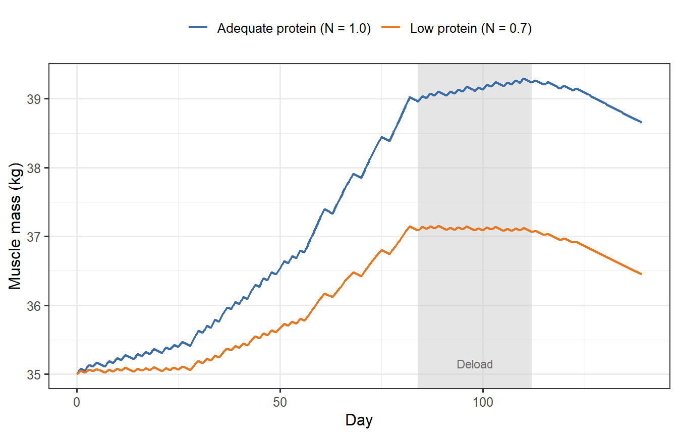
# Layer 1 — Muscle mass ODE
The simplest useful model tracks net muscle protein balance over a 20-week
training block. Training stimulus $S(t) > 0$ on session days, zero on rest days.
Nutrition adequacy $N \in [0,1]$ scales MPS: a habitual protein intake below
~1.6 g·kg$^{-1}$·day$^{-1}$ activates this penalty.
```{r muscle-ode, fig.cap="Muscle mass trajectories under adequate (blue) and insufficient (orange) protein intake during a 20-week periodised training block. The grey bar marks a 2-week deload. Even with identical training, a 30% protein shortfall costs ~0.8 kg of muscle gain — equivalent to six weeks of training."}
muscle_ode <- function(time, y, parms) {
  with(as.list(c(y, parms)), {
    day <- floor(time) + 1
    S   <- if (day <= length(schedule)) schedule[day] else 0
    dM  <- k_s * N_adeq * S - k_d * M
    list(dM)
  })
}

# 140-day periodised training schedule (arbitrary load units, 0 = rest)
make_schedule <- function(n = 140, seed = 42) {
  set.seed(seed)
  load <- numeric(n)
  for (day in seq_len(n)) {
    week <- ceiling(day / 7)
    dow  <- ((day - 1) %% 7) + 1   # day-of-week 1–7
    if      (week <=  4) { if (dow %in% c(1, 3, 5))       load[day] <- runif(1, 45, 62) }
    else if (week <=  8) { if (dow %in% c(1, 2, 4, 6))    load[day] <- runif(1, 65, 82) }
    else if (week <= 12) { if (dow %in% 1:5)               load[day] <- runif(1, 75, 92) }
    else if (week <= 16) { if (dow %in% c(1, 3, 5))        load[day] <- runif(1, 45, 62) }
    else if (week <= 18) { if (dow %in% c(1, 4))           load[day] <- runif(1, 25, 40) }
    # weeks 19–20: test/assess — no loading
  }
  load
}

schedule <- make_schedule()

parms_adeq <- list(k_s = 0.0018, k_d = 0.0008, N_adeq = 1.0,
                   schedule = schedule)
parms_low  <- list(k_s = 0.0018, k_d = 0.0008, N_adeq = 0.70,
                   schedule = schedule)

times <- seq(0, 139, by = 0.5)

run_muscle <- function(parms, M0 = 35) {
  as.data.frame(
    ode(y = c(M = M0), times = times, func = muscle_ode, parms = parms,
        method = "euler")
  )
}

mA <- run_muscle(parms_adeq)
mL <- run_muscle(parms_low)

df_m <- bind_rows(
  mutate(mA, condition = "Adequate protein (N = 1.0)"),
  mutate(mL, condition = "Low protein (N = 0.7)")
)

ggplot(df_m, aes(x = time, y = M, colour = condition)) +
  annotate("rect", xmin = 84, xmax = 112, ymin = -Inf, ymax = Inf,
           fill = "grey80", alpha = 0.5) +
  annotate("text", x = 98, y = 35.15, label = "Deload",
           size = 3, colour = "grey40") +
  geom_line(linewidth = 0.85) +
  scale_colour_manual(values = c("#3B6EA8", "#E87722")) +
  labs(x = "Day", y = "Muscle mass (kg)", colour = NULL) +
  theme_bw(base_size = 12) +
  theme(legend.position = "top")
```
---
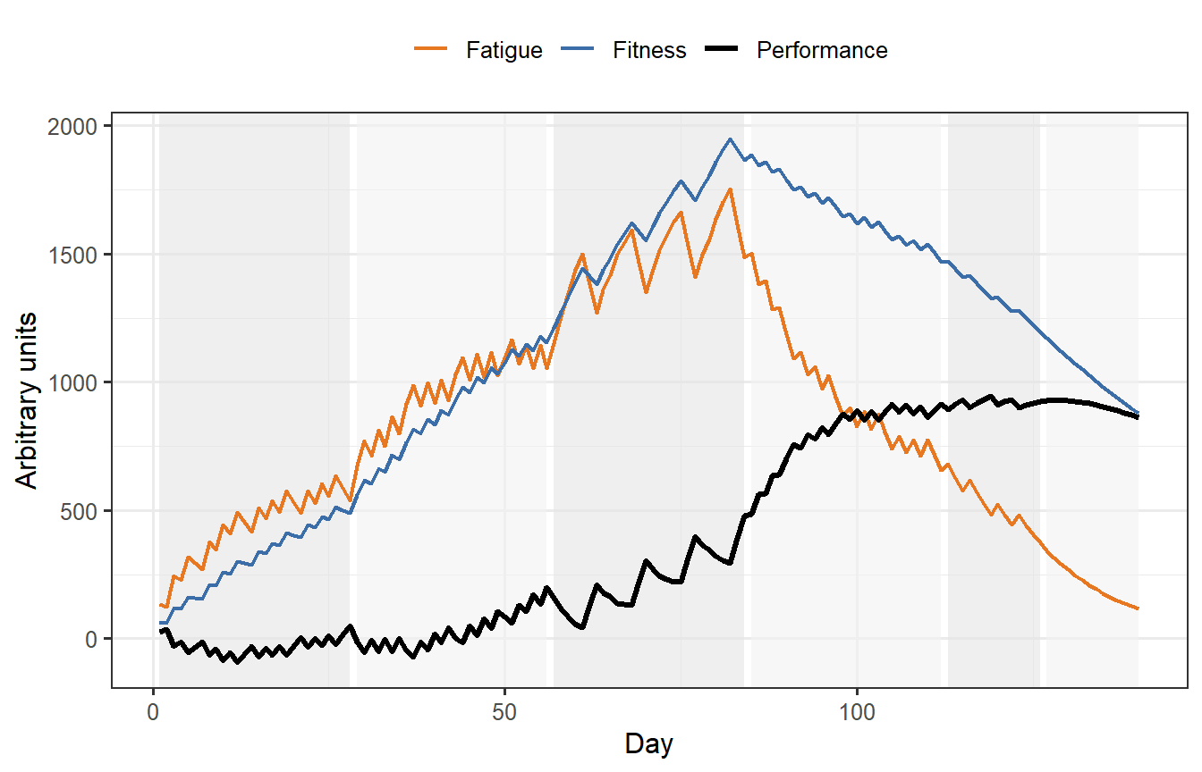
# Layer 2 — Fitness–fatigue model
The Banister model operates at the performance level and is the workhorse tool
in applied sports science. Implemented recursively, it is $O(n)$ and can be
re-fitted daily as new session data arrive — a prerequisite for a live digital
twin.
```{r banister, fig.cap="Banister fitness–fatigue simulation over 20 weeks of periodised training. Fitness (blue) accumulates through the loading phases. Fatigue (orange) spikes during the high-volume realization phase (weeks 9–12) and dissipates rapidly during the taper. Predicted performance (black) peaks after the taper when fatigue has cleared but fitness is still near its maximum."}
banister <- function(load, k1 = 1, k2 = 2.2, tau_g = 45, tau_h = 12,
                     P0 = 100) {
  n  <- length(load)
  g  <- h <- numeric(n + 1)
  ag <- exp(-1 / tau_g)
  ah <- exp(-1 / tau_h)
  for (t in seq_len(n)) {
    g[t + 1] <- ag * g[t] + k1 * load[t]
    h[t + 1] <- ah * h[t] + k2 * load[t]
  }
  data.frame(
    day  = seq_len(n),
    load = load,
    g    = g[-1],
    h    = h[-1],
    perf = P0 + g[-1] - h[-1]
  )
}

sim <- banister(schedule)

# Phase labels for annotation
phase_df <- data.frame(
  xmin  = c(1, 29, 57, 85, 113, 127),
  xmax  = c(28, 56, 84, 112, 126, 140),
  label = c("Accum.", "Intens.", "Realiz.", "Accum.", "Taper", "Peak"),
  y     = 80
)

df_b <- sim |>
  pivot_longer(c(g, h, perf),
               names_to = "component", values_to = "value") |>
  mutate(component = recode(component,
    g    = "Fitness",
    h    = "Fatigue",
    perf = "Performance"
  ))

ggplot(df_b, aes(x = day, y = value, colour = component,
                 linewidth = component)) +
  geom_rect(data = phase_df,
            aes(xmin = xmin, xmax = xmax, ymin = -Inf, ymax = Inf),
            inherit.aes = FALSE,
            fill = rep(c("grey90", "grey95"), 3), alpha = 0.6) +
  geom_line() +
  scale_colour_manual(values = c(Fitness = "#3B6EA8", Fatigue = "#E87722",
                                  Performance = "black")) +
  scale_linewidth_manual(values = c(Fitness = 0.8, Fatigue = 0.8,
                                     Performance = 1.1)) +
  labs(x = "Day", y = "Arbitrary units", colour = NULL,
       linewidth = NULL) +
  theme_bw(base_size = 12) +
  theme(legend.position = "top")
```
---
# Layer 3 — Virtual trainee cohort
The critical insight motivating a digital twin over a population-average
prescription is that individuals differ substantially in their fitness and fatigue
time constants. A high $k_2 / k_1$ ratio means more fatigue per unit of load —
these individuals need longer recovery periods. A long $\tau_g$ means fitness is
retained longer — these individuals benefit more from detraining periods.
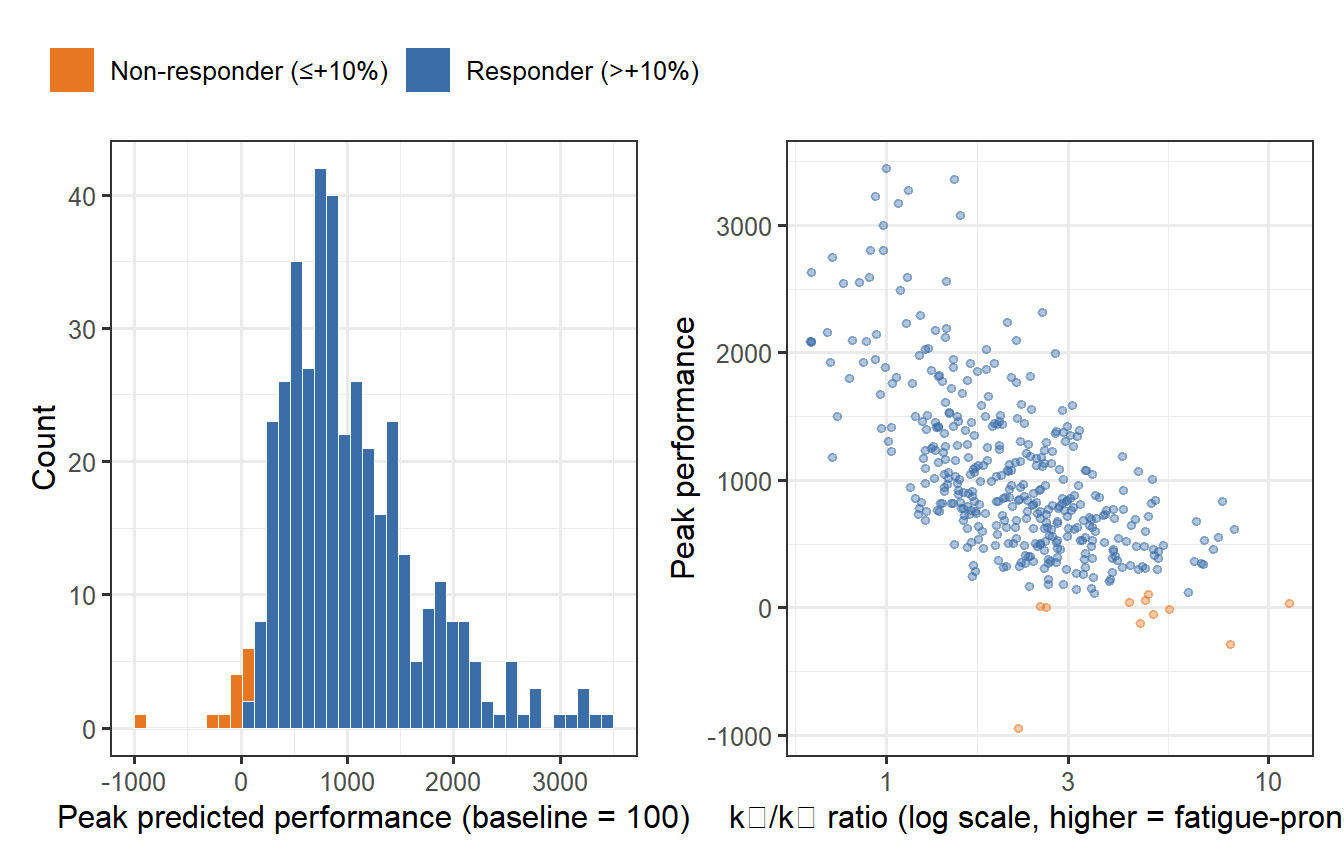
```{r virtual-cohort, fig.cap="Predicted peak performance across 400 virtual trainees after the same 20-week programme. Individual variation in Banister parameters (τ_g, τ_h, k1, k2) produces a wide performance distribution. Some individuals peak 15–20% above baseline; others barely improve — the same programme, radically different outcomes."}
set.seed(99)
n_vt <- 400

# Log-normal individual parameters
tau_g_i <- exp(rnorm(n_vt, log(45), 0.25))
tau_h_i <- exp(rnorm(n_vt, log(12), 0.30))
k1_i    <- exp(rnorm(n_vt, log(1.0), 0.35))
k2_i    <- exp(rnorm(n_vt, log(2.2), 0.35))

peak_perf <- mapply(function(tg, th, k1, k2) {
  sim_i <- banister(schedule, k1 = k1, k2 = k2,
                    tau_g = tg, tau_h = th, P0 = 100)
  max(sim_i$perf[sim_i$day >= 120])   # peak in final 20 days
}, tau_g_i, tau_h_i, k1_i, k2_i)

df_vt <- data.frame(
  peak     = peak_perf,
  k_ratio  = k2_i / k1_i,
  responder = ifelse(peak_perf > 110, "Responder (>+10%)", "Non-responder (≤+10%)")
)

p_hist <- ggplot(df_vt, aes(x = peak, fill = responder)) +
  geom_histogram(bins = 40, colour = "white", linewidth = 0.15) +
  scale_fill_manual(values = c("Responder (>+10%)" = "#3B6EA8",
                                "Non-responder (≤+10%)" = "#E87722")) +
  labs(x = "Peak predicted performance (baseline = 100)",
       y = "Count", fill = NULL) +
  theme_bw(base_size = 12) +
  theme(legend.position = "top")

p_scatter <- ggplot(df_vt, aes(x = k_ratio, y = peak, colour = responder)) +
  geom_point(alpha = 0.4, size = 1.2) +
  scale_colour_manual(values = c("Responder (>+10%)" = "#3B6EA8",
                                  "Non-responder (≤+10%)" = "#E87722")) +
  scale_x_log10() +
  labs(x = "k₂/k₁ ratio (log scale, higher = fatigue-prone)",
       y = "Peak performance", colour = NULL) +
  theme_bw(base_size = 12) +
  theme(legend.position = "none")

p_hist + p_scatter
```
About 25–30% of virtual trainees fail to exceed a 10% performance gain despite
completing the full programme — a proportion strikingly consistent with
empirical estimates of non-response to resistance training in randomised trials.
The scatter plot reveals the mechanism: high $k_2/k_1$ individuals accumulate
fatigue faster than fitness, staying suppressed through the loading phases and
never fully recovering during the brief taper.
---
# Business opportunity assessment
## The gap in the market
The fitness technology market is large and growing — wearables, coaching apps,
and gym software collectively represent tens of billions of dollars in annual
revenue. Yet almost none of it runs mechanistic models. Existing products fall
into two categories:
**Heuristic load monitoring** (WHOOP, OURA, Garmin, Polar): compute acute and
chronic training load proxies from heart rate and movement data. These track
*symptoms* of training stress but cannot predict individual adaptation or
optimise a programme prospectively. The underlying model is essentially a
smoothed moving average — no parameters to personalise, no differential
equations, no counterfactual reasoning.
**AI-based recommendation** (future.com, Freeletics, various LLM-powered apps):
use machine learning on population data to suggest workouts. These are
correlational and cannot simulate *what would happen if* training load changes.
They cannot model the non-responder problem or sarcopenia trajectory.
The gap is mechanistic individualisation: a parametric model fitted to a
specific person's longitudinal data that can be queried prospectively. This is
what a muscle digital twin provides.
## Where the value is highest
**1. Sarcopenia prevention and early intervention** is the most defensible
near-term opportunity. A twin calibrated from routine biomarkers (serum
creatinine, appendicular lean mass from DEXA, grip strength) and wearable
activity data could predict 5-year sarcopenia trajectory with clinically
actionable precision [@cruzjentoft2019]. The target buyer is health systems and
insurers, not individuals — B2B pricing makes unit economics tractable even at
low volumes. Regulatory pathway (digital therapeutic or Software as a Medical
Device) is demanding but creates a durable moat.
**2. Drug development** represents the highest-value single application. Phase 3
trials for sarcopenia pharmacotherapies (myostatin inhibitors, selective androgen
receptor modulators, GDF-11 analogues) require years of follow-up and large
sample sizes because the primary endpoint — change in lean mass or gait speed —
has high inter-individual variance. A validated muscle digital twin used as a
prognostic covariate (analogous to PROCOVA for PROCOVA in other indications)
could reduce required sample size by 20–40%, saving tens of millions per trial.
This is directly analogous to what we explored for vaccine trials in this series:
the same FDA MIDD framework that encourages model-based vaccine development
applies here.
**3. The responder/non-responder problem** is underappreciated commercially. The
virtual cohort simulation above shows that ~25% of people who complete a
structured programme gain little. In a 12-week personalised training programme
priced at \$200–500, a non-responder is an at-risk churner and a negative review.
Early identification of non-responders (from 3–4 weeks of biomarker data and
wearables) and re-routing them to a modified protocol has direct economic value
for any subscription fitness business. No current product does this
mechanistically.
**4. Corporate wellness** is an underexplored distribution channel. Employers pay
substantial costs for musculoskeletal injuries (back pain, repetitive strain),
which are the leading cause of workplace disability claims. Resistance training
demonstrably reduces injury risk, but generic programmes have poor adherence.
Individualised digital twins embedded in employer benefit platforms could improve
adherence and justify outcomes-based pricing.
## The data flywheel and competitive moat
The central challenge for any muscle digital twin business is the **cold-start
problem**: Banister and ODE parameters are only identifiable after 4–8 weeks of
longitudinal measurements on the individual. This is not a fatal flaw — it is a
structural moat. Once a twin is calibrated, switching costs are high (all that
historical data lives in one system). The competitor who accumulates the largest
database of individual trajectories will have the best priors for initialising
new users, compressing the calibration period.
The realistic near-term business model is therefore a *professional tier*
(coaches, physical therapists, sports scientists) who tolerate a calibration
period in exchange for model-informed programming — analogous to how
pharmacometrics modellers use NONMEM or Monolix in drug development.
Consumer direct-to-market will follow once the calibration barrier is
lowered by better population priors.
---
# Potential directions
## Precision nutrition integration
Muscle protein synthesis is rate-limited by leucine availability at the
ribosome. The per-meal leucine threshold (~2–3 g to maximally stimulate MPS)
is relatively conserved across individuals, but the *dose–response curve* for
protein amount, timing relative to training, and distribution across meals varies.
A twin that couples the training stimulus model with a pharmacokinetic model
of dietary amino acid absorption would enable genuinely personalised protein
prescriptions — not population RDA recommendations but individual optimisation
of meal size, timing, and protein source given a specific training schedule.
The data requirements are modest: a 7-day diet diary, body composition, and
2–3 blood draws.
## Ageing and anabolic resistance
Older adults exhibit *anabolic resistance*: a blunted MPS response to both
protein and exercise stimulus, requiring higher doses of both to achieve the same
adaptive response. In ODE terms, $k_s$ declines with age while $k_d$ is
relatively preserved — a progressively unfavourable balance. A longitudinal
model that tracks this ratio over decades, calibrated to periodic biomarker
measurements, could identify when anabolic resistance becomes clinically
significant and when pharmacological augmentation (e.g. leucine supplementation,
β-hydroxy-β-methylbutyrate, or in higher-risk settings, clinical agents) becomes
warranted. This is the most direct connection between a muscle digital twin and
clinical practice.
## Rehabilitation and injury recovery
Post-surgical muscle atrophy (e.g. following ACL reconstruction or hip
arthroplasty) follows the same ODE structure but with a negative stimulus for
the early immobilisation phase and constrained recovery trajectories. A twin that
is calibrated pre-surgery could model the expected atrophy, predict the
post-rehabilitation trajectory, and flag patients who are recovering slower than
predicted — enabling early re-intervention. Physical therapy is currently driven
almost entirely by protocol adherence and subjective assessments; a continuous
model-predicted trajectory would change the clinical conversation.
## Multi-scale extension
The post on multiscale digital twins in this series described a three-scale
pipeline for vaccine trials: molecular → individual → population. The same
architecture applies here:
| Scale | Model | Key output |
|---|---|---|
| Molecular | mTOR signalling ODE (substrate, kinase, effector) | MPS rate coefficient $k_s(t)$ |
| Cellular | Satellite cell activation and fibre hypertrophy | Cross-sectional area per fibre type |
| Organ | Whole-muscle mass ODE + Banister performance layer | Force output, lean mass |
| System | Metabolic and cardiovascular coupling | VO₂max, insulin sensitivity |
Coupling molecular mTOR dynamics (Scale 1) to the muscle mass ODE (Scale 2) and
the Banister performance layer (Scale 3) would allow a fully mechanistic twin
that connects a specific training session, through signalling kinetics, to
measured force output days later. No such model is currently in clinical use,
but the biological building blocks exist in the academic literature [@bodine2001].
---
# Limitations and caveats
The models here are intentionally minimal. Real hypertrophy involves fibre-type
composition shifts (Type I vs Type IIx), satellite cell-mediated myonuclear
addition (a prerequisite for substantial hypertrophy that is not captured by a
single $M$ compartment), vascularisation changes, and tendon remodelling on
longer timescales.
The Banister model is also phenomenological rather than mechanistic: it fits a
training-to-performance transfer function without encoding the biological pathway.
Its parameters ($\tau_g$, $\tau_h$, $k_1$, $k_2$) are not directly measurable
from biomarkers — they must be inferred from a time series of load and
performance, which requires at least 4–8 weeks of data and creates
identifiability challenges when the programme has low variability in load.
For clinical or regulatory use, the validation bar is high: the FDA expects
prospective validation on held-out cohorts with pre-specified decision criteria —
the same standard discussed in the vaccine trial post in this series. Building
that evidence base is the primary scientific challenge for the field.
---
# References {.unnumbered}
::: {#refs}
:::
```{r session-info, echo=FALSE}
sessionInfo()
```