---
title: "Multiscale Modelling for Digital Twins in Vaccine Trials"
subtitle: "A three-scale R pipeline: viral dynamics → antibody kinetics → population trial outcomes"
author: "Jong-Hoon Kim"
date: "2026-04-22"
categories: [digital twin, multiscale, ODE, R, vaccine, infectious disease]
bibliography: references.bib
csl: https://www.zotero.org/styles/vancouver
format:
html:
toc: true
toc-depth: 3
code-fold: true
code-tools: true
number-sections: true
fig-width: 7
fig-height: 4.5
fig-align: center
knitr:
opts_chunk:
message: false
warning: false
fig.retina: 2
---
```{r setup, include=FALSE}
library(deSolve)
library(ggplot2)
library(dplyr)
library(tidyr)
library(patchwork)
```
# Why multiple scales?
The outcome of a vaccine trial depends on processes that span at least three orders of magnitude in time and space: molecular events inside a single cell, the kinetics of an individual's immune system, and the spread of a pathogen through a population. A *multiscale digital twin* is a computational stack that couples models at each of these scales so that trial-level predictions inherit uncertainty from every scale below [@masison2021].
This post builds such a stack in R. Each section implements one scale as an ODE system, connects its outputs to the next scale, and visualises the resulting dynamics. The goal is a *working pipeline* you can inspect, modify, and reason about.
| Scale | Model | Key output |
|---|---|---|
| 1 — Within-host | Target cell ODEs | Viral load trajectory |
| 2 — Immunological | Antigen–antibody ODEs | Titre at challenge; waning rate |
| 3 — Population | SIR with heterogeneous VE | Attack rate in trial arms |
---
# Scale 1 — Within-host viral dynamics
## The target cell model
The *target cell limited* model [@perelson1996] tracks three populations:
$$
\frac{dT}{dt} = \lambda - d_T T - \beta V T
$$
$$
\frac{dI}{dt} = \beta V T - \delta I
$$
$$
\frac{dV}{dt} = p\,I - c\,V
$$
$T$ = uninfected target cells (e.g. airway epithelial cells), $I$ = productively infected cells, $V$ = free virus (virions/mL). The within-host basic reproductive number is $R_0^w = \beta T_0 p \,(c\,\delta)^{-1}$.
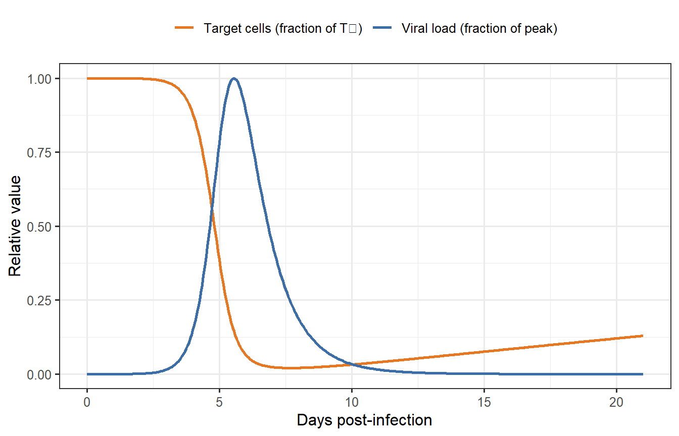
```{r scale1-single, fig.cap="Single within-host simulation. Viral load (blue) peaks around day 4–5 as infected cells expand, then collapses as target cells are depleted and virus is cleared. Target cells (orange) partially recover after the acute phase."}
tcm <- function(t, y, parms) {
  with(as.list(c(y, parms)), {
    dT <-  lambda - d_T * T - beta * V * T
    dI <-  beta  * V * T   - delta * I
    dV <-  p * I            - c    * V
    list(c(dT, dI, dV))
  })
}

# Parameters for a generic respiratory virus (for illustration)
# R0_within = beta * T0 * p / (c * delta) = 5e-8 * 1e7 * 50 / 5 = 5
parms0 <- c(
  lambda = 1e5,   # target-cell production (/day); T* = lambda/d_T = 1e7
  d_T    = 0.01,  # background death rate (/day)
  beta   = 5e-8,  # infection rate constant (mL/virion/day)
  delta  = 1.0,   # infected-cell clearance (/day)
  p      = 50,    # viral burst size (virions/cell/day)
  c      = 5.0    # viral clearance rate (/day)
)

y0    <- c(T = 1e7, I = 100, V = 0)   # I0 = 100 initially infected cells
times <- seq(0, 21, by = 0.05)

out0 <- as.data.frame(ode(y = y0, times = times, func = tcm, parms = parms0))

df1 <- out0 |>
  select(time, T, V) |>
  mutate(
    T = T / 1e7,           # fraction of initial target cells
    V = V / max(V)         # fraction of peak viral load
  ) |>
  pivot_longer(c(T, V), names_to = "variable", values_to = "value") |>
  mutate(variable = recode(variable,
    T = "Target cells (fraction of T₀)",
    V = "Viral load (fraction of peak)"
  ))

ggplot(df1, aes(x = time, y = value, colour = variable)) +
  geom_line(linewidth = 0.9) +
  scale_colour_manual(values = c("#E87722", "#3B6EA8")) +
  labs(x = "Days post-infection", y = "Relative value", colour = NULL) +
  theme_bw(base_size = 12) +
  theme(legend.position = "top")
```
## Effect of immune clearance rate
The infected-cell clearance rate $\delta$ encodes the combined effect of cytotoxic T-cell killing, innate immune pressure, and apoptosis. People differ in $\delta$: stronger cellular immunity clears infected cells faster, limiting peak viraemia.
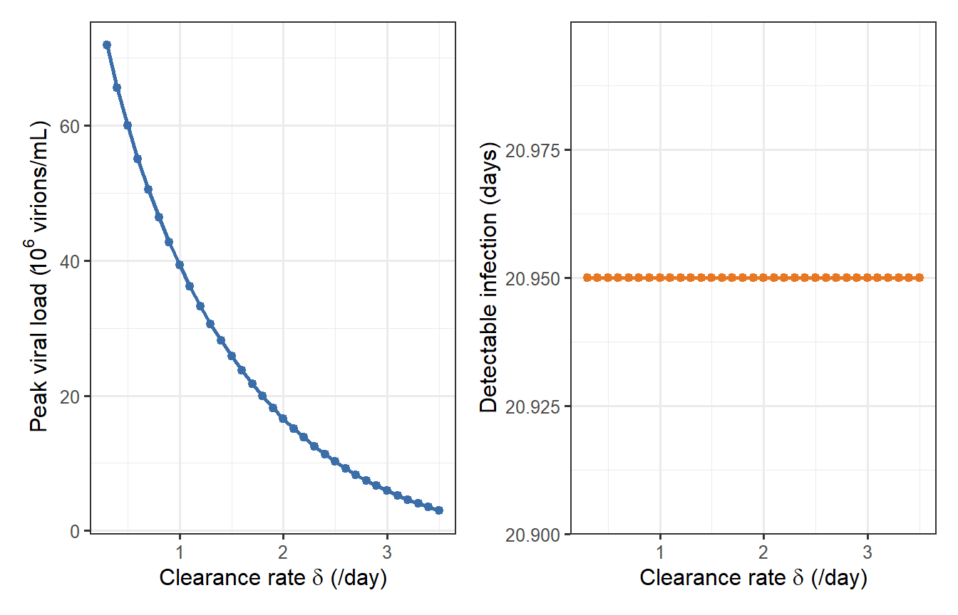
```{r scale1-sweep, fig.cap="Effect of varying the infected-cell clearance rate δ on peak viral load (left) and the duration virus is detectable above 1 virion/mL (right). The nonlinear collapse above δ ≈ 1.5 /day illustrates why a modest boost in cellular immunity can dramatically reduce viraemia."}
delta_vals <- seq(0.3, 3.5, by = 0.1)

sweep_res <- lapply(delta_vals, function(d) {
  p_i        <- parms0
  p_i["delta"] <- d
  out_i      <- as.data.frame(
    ode(y = y0, times = times, func = tcm, parms = p_i)
  )
  above    <- out_i$V > 1
  duration <- if (any(above)) diff(range(out_i$time[above])) else 0
  data.frame(delta = d, peak_V = max(out_i$V), duration = duration)
})
sw <- bind_rows(sweep_res)

p_pk <- ggplot(sw, aes(x = delta, y = peak_V / 1e6)) +
  geom_line(colour = "#3B6EA8", linewidth = 0.9) +
  geom_point(colour = "#3B6EA8", size = 1.8) +
  labs(x = expression(paste("Clearance rate ", delta, " (/day)")),
       y = expression(paste("Peak viral load (", 10^6, " virions/mL)"))) +
  theme_bw(base_size = 12)

p_dur <- ggplot(sw, aes(x = delta, y = duration)) +
  geom_line(colour = "#E87722", linewidth = 0.9) +
  geom_point(colour = "#E87722", size = 1.8) +
  labs(x = expression(paste("Clearance rate ", delta, " (/day)")),
       y = "Detectable infection (days)") +
  theme_bw(base_size = 12)

p_pk + p_dur
```
This parameter sweep motivates the virtual patient concept: if individuals draw $\delta$ from a distribution rather than a single value, the resulting viral load trajectories span a wide range, producing the population-level heterogeneity that Scale 2 and Scale 3 must represent.
---
# Scale 2 — Vaccine-induced antibody kinetics
## Antigen-driven antibody model
After vaccination, antigen is cleared while simultaneously driving B-cell differentiation and antibody secretion. A two-compartment model captures the essentials:
$$
\frac{dAg}{dt} = -k_{Ag}\,Ag
$$
$$
\frac{dAb}{dt} = r_{Ab}\,Ag - d_{Ab}\,Ab
$$
$Ag$ = antigen (normalised dose units), $Ab$ = serum antibody titre (AU/mL). With $Ag(0)=1$, $Ab(0)=0$, the analytical solution is:
$$
Ab(t) = \frac{r_{Ab}}{k_{Ag}-d_{Ab}}\bigl(e^{-d_{Ab}t}-e^{-k_{Ag}t}\bigr)
$$
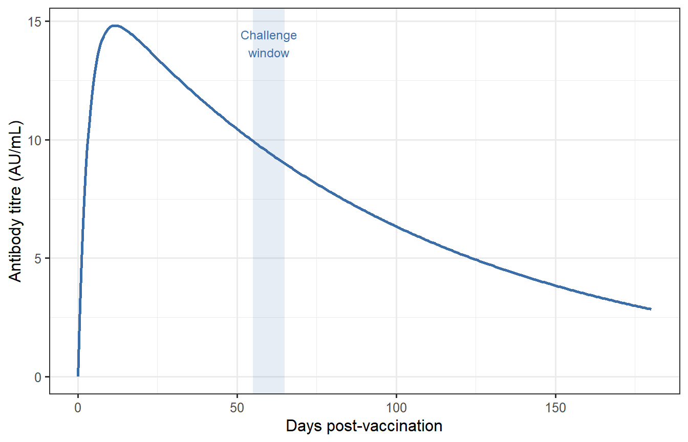
Titre peaks at $t^{*} = \ln(k_{Ag}/d_{Ab})\,/\,(k_{Ag}-d_{Ab})$, typically 10–21 days, then wanes as $e^{-d_{Ab}t}$ dominates.
```{r scale2-single, fig.cap="Antibody kinetics for a single vaccinee. Titre peaks near day 14 and wanes slowly over months. The shaded band marks the 60-day challenge window used in Scale 3."}
Ab_t <- function(t, r_Ab = 5, d_Ab = 0.01, k_Ag = 0.3) {
  r_Ab / (k_Ag - d_Ab) * (exp(-d_Ab * t) - exp(-k_Ag * t))
}

t_vac <- seq(0, 180, by = 0.5)
df2a  <- data.frame(time = t_vac, titre = Ab_t(t_vac))

ggplot(df2a, aes(x = time, y = titre)) +
  annotate("rect", xmin = 55, xmax = 65, ymin = -Inf, ymax = Inf,
           fill = "#3B6EA8", alpha = 0.12) +
  geom_line(colour = "#3B6EA8", linewidth = 0.9) +
  annotate("text", x = 60, y = max(df2a$titre) * 0.95,
           label = "Challenge\nwindow", size = 3.2, hjust = 0.5,
           colour = "#3B6EA8") +
  labs(x = "Days post-vaccination", y = "Antibody titre (AU/mL)") +
  theme_bw(base_size = 12)
```
## Virtual patient cohort
Two parameters capture the main axes of inter-individual variation:
- $r_{Ab}$: immune responsiveness (B-cell clone size, adjuvant response)
- $d_{Ab}$: waning rate (long-lived plasma-cell survival, isotype class)
We sample 500 virtual vaccinees from log-normal distributions and extract each individual's titre at day 60 — a plausible mid-trial challenge time.
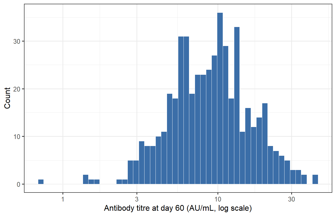
```{r scale2-cohort, fig.cap="Distribution of antibody titres at the 60-day challenge window across 500 virtual patients. The log scale reveals the right-skewed distribution typical of clinical immunogenicity data. Variation arises from individual differences in immune responsiveness and antibody waning."}
set.seed(42)
n_vp <- 500

r_Ab_i <- exp(rnorm(n_vp, log(5),    0.55))  # ~55% CV in responsiveness
d_Ab_i <- exp(rnorm(n_vp, log(0.01), 0.40))  # ~40% CV in waning rate

titre_60 <- pmax(
  mapply(Ab_t, t = 60, r_Ab = r_Ab_i, d_Ab = d_Ab_i),
  0.01   # numerical floor
)

ggplot(data.frame(titre = titre_60), aes(x = titre)) +
  geom_histogram(bins = 50, fill = "#3B6EA8", colour = "white",
                 linewidth = 0.2) +
  scale_x_log10() +
  labs(x = "Antibody titre at day 60 (AU/mL, log scale)", y = "Count") +
  theme_bw(base_size = 12)
```
The distribution is approximately log-normal, consistent with observed immunogenicity data for licensed vaccines. The two-fold range from 5th to 95th percentile reflects the biological reality that the same vaccine produces widely varying responses across individuals.
---
# Scale 3 — Population trial outcome
## From titre to individual protection
The antibody–protection relationship is well described by a Hill function:
$$
\text{VE}_i = \frac{T_i^k}{T_i^k + \text{EC}_{50}^k}
$$
where $T_i$ is individual $i$'s titre at challenge, $\text{EC}_{50}$ is the titre giving 50% protection, and $k$ governs steepness. Setting $\text{EC}_{50} = \text{median}(T_i)$ ensures that the median virtual patient has 50% protection — a conservative but transparent calibration choice.
## Analytic attack rate
For an SIR epidemic, the final attack rate satisfies the implicit equation:
$$
1 - \text{AR} = \exp\!\bigl(-R_0^{\text{eff}}\cdot\text{AR}\bigr), \qquad
R_0^{\text{eff}} = R_0\,(1 - \bar{\text{VE}})
$$
where $\bar{\text{VE}} = n^{-1}\sum_i \text{VE}_i$. This avoids running one ODE system per trial replicate while preserving the nonlinear epidemic threshold behaviour.
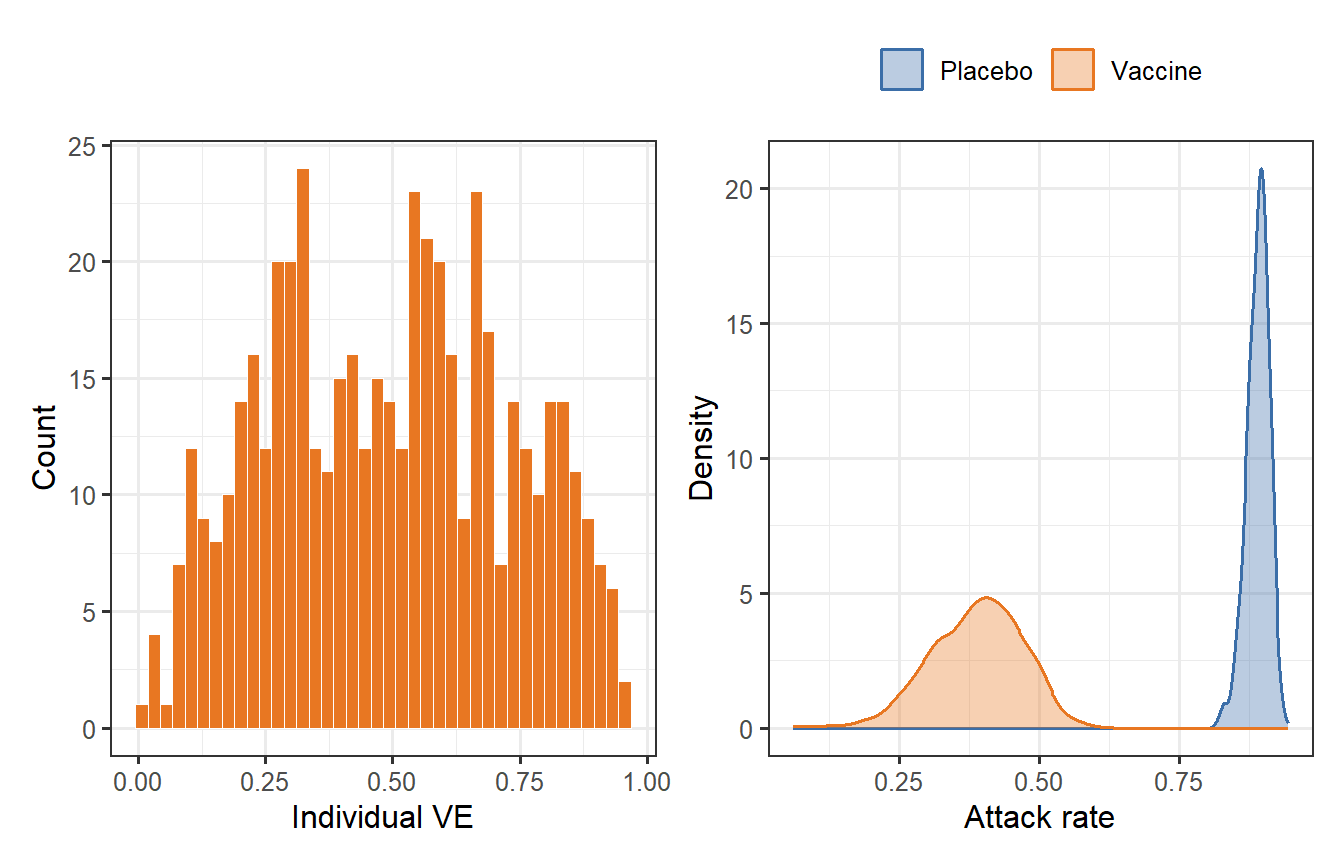
```{r scale3, fig.cap="Scale 3 outputs. Left: individual VE distribution across the 500 virtual vaccinees, arising directly from the titre distribution in Scale 2. Right: attack-rate densities across 1000 bootstrapped trial replicates (200 participants per arm). The vaccinated arm (orange) is shifted far left of the placebo arm (blue), with additional spread from VE heterogeneity."}
EC50 <- median(titre_60)
k    <- 2
VEi  <- titre_60^k / (titre_60^k + EC50^k)

ar_solve <- function(mean_VE, R0 = 2.5) {
  R0_eff <- R0 * (1 - mean_VE)
  if (R0_eff <= 1) return(0)
  uniroot(function(ar) 1 - ar - exp(-R0_eff * ar),
          interval = c(1e-8, 1 - 1e-8))$root
}

set.seed(7)
n_trial <- 200
n_rep   <- 1000

vacc_ar <- replicate(n_rep, {
  idx  <- sample(n_vp, n_trial, replace = FALSE)
  R0_i <- rnorm(1, 2.5, 0.15)
  ar_solve(mean(VEi[idx]), R0_i)
})

placebo_ar <- replicate(n_rep, {
  ar_solve(0, rnorm(1, 2.5, 0.15))
})

p_ve <- ggplot(data.frame(VE = VEi), aes(x = VE)) +
  geom_histogram(bins = 40, fill = "#E87722", colour = "white",
                 linewidth = 0.2) +
  labs(x = "Individual VE", y = "Count") +
  theme_bw(base_size = 12)

df3 <- bind_rows(
  data.frame(arm = "Vaccine", ar = vacc_ar),
  data.frame(arm = "Placebo", ar = placebo_ar)
)

p_ar <- ggplot(df3, aes(x = ar, fill = arm, colour = arm)) +
  geom_density(alpha = 0.35, linewidth = 0.7) +
  scale_fill_manual(values  = c(Vaccine = "#E87722", Placebo = "#3B6EA8")) +
  scale_colour_manual(values = c(Vaccine = "#E87722", Placebo = "#3B6EA8")) +
  labs(x = "Attack rate", y = "Density", fill = NULL, colour = NULL) +
  theme_bw(base_size = 12) +
  theme(legend.position = "top")

p_ve + p_ar
```
---
# Cross-scale sensitivity analysis
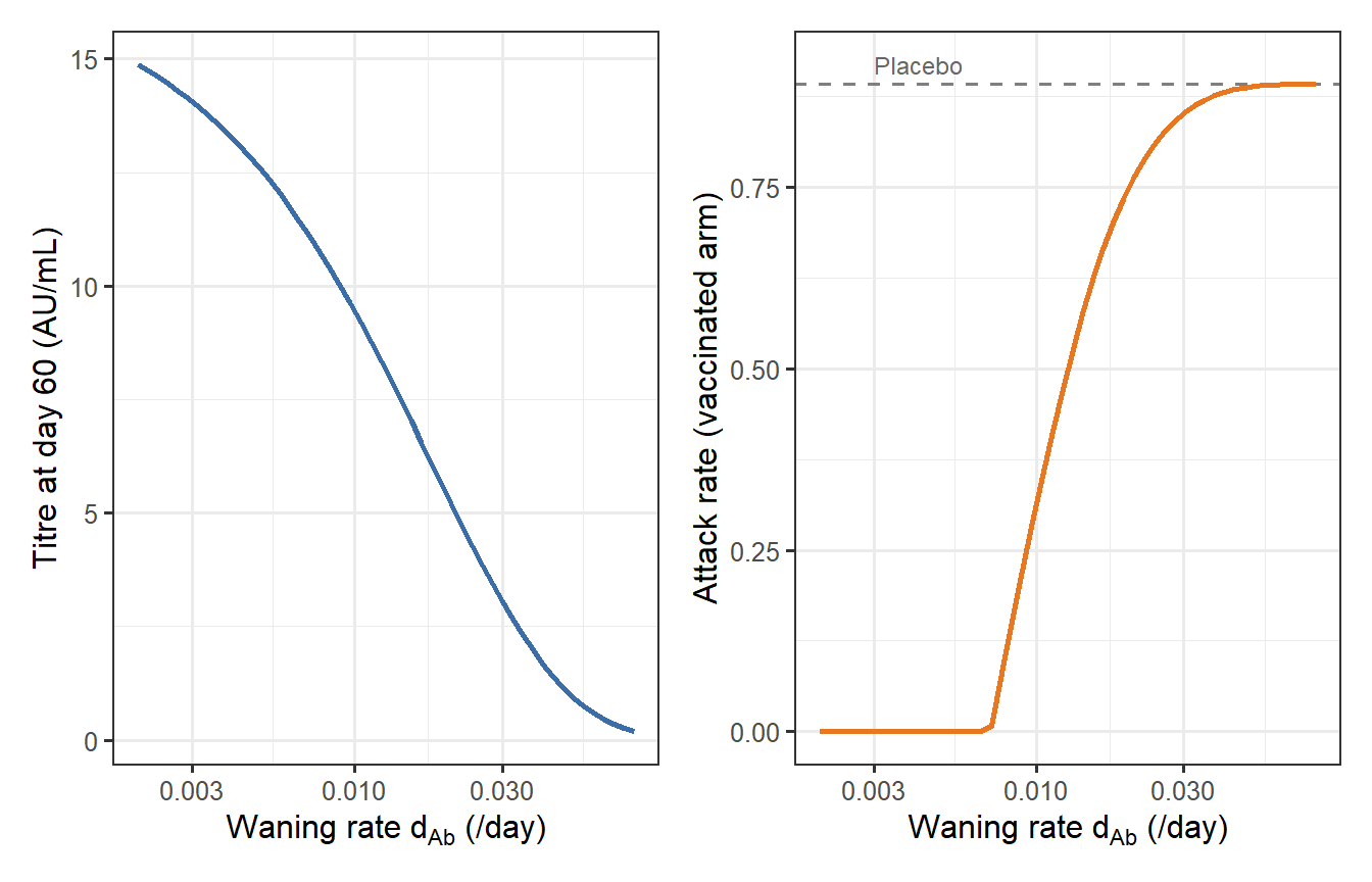
A key virtue of a multiscale pipeline is that you can trace how uncertainty at one scale propagates to outcomes at another. Here we sweep the antibody waning rate $d_{Ab}$ (Scale 2) across a physiologically plausible range and ask: how does it affect the attack rate in the vaccinated arm (Scale 3)?
```{r cross-scale, fig.cap="Cross-scale propagation: how the Scale 2 waning rate d_Ab drives the Scale 3 trial outcome. Left: titre at the 60-day challenge window collapses as waning accelerates. Right: corresponding attack rate in the vaccinated arm rises toward the placebo level (grey dashed line, R₀ = 2.5). The inflection near d_Ab ≈ 0.01 /day (antibody half-life ∼ 70 days) marks the critical waning threshold for this vaccine and challenge scenario."}
d_Ab_range <- exp(seq(log(0.002), log(0.08), length.out = 50))

cross <- lapply(d_Ab_range, function(d) {
  t_i   <- max(Ab_t(60, r_Ab = 5, d_Ab = d), 0.01)
  ve_i  <- t_i^k / (t_i^k + EC50^k)
  ar_i  <- ar_solve(ve_i, R0 = 2.5)
  data.frame(d_Ab = d, titre = t_i, ar = ar_i)
})
cr <- bind_rows(cross)

placebo_ref <- ar_solve(0, 2.5)

p_cs1 <- ggplot(cr, aes(x = d_Ab, y = titre)) +
  geom_line(colour = "#3B6EA8", linewidth = 0.9) +
  scale_x_log10() +
  labs(x = expression(paste("Waning rate ", d[Ab], " (/day)")),
       y = "Titre at day 60 (AU/mL)") +
  theme_bw(base_size = 12)

p_cs2 <- ggplot(cr, aes(x = d_Ab, y = ar)) +
  geom_hline(yintercept = placebo_ref, linetype = "dashed",
             colour = "grey50") +
  geom_line(colour = "#E87722", linewidth = 0.9) +
  annotate("text", x = 0.003, y = placebo_ref * 1.03,
           label = "Placebo", size = 3.2, colour = "grey40", hjust = 0) +
  scale_x_log10() +
  labs(x = expression(paste("Waning rate ", d[Ab], " (/day)")),
       y = "Attack rate (vaccinated arm)") +
  theme_bw(base_size = 12)

p_cs1 + p_cs2
```
When $d_{Ab}$ is small (slow waning), titres remain above EC$_{50}$ at day 60 and the vaccinated arm is well protected. As waning accelerates, titres fall below EC$_{50}$ and trial attack rate converges to the placebo level. This curve is directly actionable for trial design: it identifies the minimum waning rate that the vaccine must achieve to preserve measurable efficacy at a given challenge time.
---
# Discussion
## What makes this a digital twin?
Three features distinguish this pipeline from a conventional transmission model:
1. **Individualisation.** Each virtual patient has their own $(r_{Ab},\, d_{Ab})$, producing a titre distribution rather than a point estimate. The trial outcome inherits this individual-level variability directly.
2. **Explicit scale coupling.** Scale 2 outputs feed into Scale 3 analytically, and the cross-scale analysis runs the pipeline in reverse — from a target attack rate down to the required titre and then to the required waning rate. Bidirectional reasoning is what separates a digital twin from a forward-only simulation.
3. **Counterfactual control arm.** The placebo arm is generated by setting $\overline{\text{VE}} = 0$ in the same SIR model. This counterfactual is the regulatory anchor that sponsors submit to FDA/EMA under the MIDD program [@fda2020midd].
## Limitations of this illustration
- **Decoupled Scale 1.** In a full multiscale twin, the viral dynamics model (Scale 1) would set initial conditions for Scale 2: the antigen dose reaching lymph nodes is a function of the viral inoculum and the innate immune response at the injection site. Coupling these requires a more elaborate interfacing layer, as implemented in the mRNA vaccine QSP models of Dasti et al. [@dasti2025].
- **Steady-state immunity.** The model fixes challenge at a single time point (day 60). A realistic twin would draw challenge time from the epidemic curve — itself a Scale 3 output — creating a feedback loop that the present pipeline ignores.
- **Homogeneous mixing.** The SIR final-size approximation assumes random contact. Age structure, household clustering, or healthcare-worker exposure would each shift the attack rate curve and require additional scales [@niarakis2024].
## Extensions
The pipeline is modular by design: swapping Scale 1 from a generic respiratory model to an influenza-specific or SARS-CoV-2-specific parameterisation [@perelson1996] requires changing only that block. Similarly, Scale 3 can be upgraded from a homogeneous SIR to an age-stratified SEIR without touching Scales 1 or 2. This modularity — formalised by Masison et al. [@masison2021] — is what makes multiscale digital twins tractable despite their apparent complexity.
Physics-informed neural networks [@raissi2019] offer a complementary direction: rather than specifying between-scale mappings analytically, a neural network trained on multi-scale longitudinal data can learn them from observations, at the cost of interpretability but with potentially higher accuracy when mechanistic knowledge is incomplete.
---
# References {.unnumbered}
::: {#refs}
:::
```{r session-info, echo=FALSE}
sessionInfo()
```