---
title: "Correlates of Protection"
subtitle: "Linking antibody titres to infection risk — Post 2 in the Digital Twins for Vaccine Trials series"
author: "Jong-Hoon Kim"
date: "2026-04-22"
categories: [digital twin, vaccine, correlate of protection, immunology, R]
bibliography: references.bib
csl: https://www.zotero.org/styles/vancouver
format:
html:
toc: true
toc-depth: 3
code-fold: true
code-tools: true
number-sections: true
fig-width: 7
fig-height: 4.5
fig-align: center
knitr:
opts_chunk:
message: false
warning: false
fig.retina: 2
---
```{r setup, include=FALSE}
library(deSolve)
library(ggplot2)
library(dplyr)
library(tidyr)
library(patchwork)
theme_set(theme_bw(base_size = 12))
# Within-host ODE from Post 1 (reproduced here for self-containment)
withinhost_vax <- function(t, state, parms) {
with(as.list(c(state, parms)), {
list(c(
-delta_A * A,
kS * A * (1 + phi_S * M) - delta_S * S,
kL * A * (1 + phi_L * M) - delta_L * L,
eps * S - delta_M * M,
rS * S + rL * L - delta_Ab * Ab
))
})
}
parms_wh <- c(
delta_A = 0.30, delta_S = 0.15, delta_L = 0.003, delta_M = 0.004,
delta_Ab = 0.018, kS = 5.0, kL = 0.5, rS = 2.0, rL = 5.0,
eps = 0.05, phi_S = 3.0, phi_L = 8.0
)
state0 <- c(A = 1, S = 0, L = 0, M = 0, Ab = 0)
times_wh <- seq(0, 365, by = 0.5)
dose2 <- data.frame(var = "A", time = 21, value = 1, method = "add")
out_pb <- as.data.frame(ode(y = state0, times = times_wh,
func = withinhost_vax, parms = parms_wh,
events = list(data = dose2)))
```
# The bridge from immune model to clinical endpoint
[Post 1](https://www.jonghoonk.com/blog/posts/digital_twin_within_host/) built a within-host ODE model that predicts the antibody titre trajectory $\text{Ab}(t)$ for a vaccinated individual. We can run that model for any individual whose parameters we know and get a full 12-month titre curve.
But the question a clinical trial cares about is not *what is this person's titre?* — it is *will this person get infected?* Connecting the two requires a **correlate of protection** (CoP): a relationship between an immune measurement and the probability of being protected from infection.
The CoP is the second essential building block of a vaccine digital twin. Without it, the within-host model produces immunological outputs that float free of any clinical meaning. With it, every point on the antibody trajectory becomes a probability of protection at that moment in time — exactly what trial simulation requires.
---
# What is a correlate of protection?
Plotkin defined a correlate of protection as "an immune response that is statistically interchangeable with protection" [@plotkin2010]. The formal statistical version, due to Prentice [@prentice1989] and later refined by Qin et al. [@qin2007], requires the immune marker to capture all of the treatment effect on the clinical outcome. Plotkin and Gilbert later distinguished [@plotkin2012]:
- **Correlate of protection (CoP)**: a marker that statistically predicts protection, without necessarily causing it.
- **Mechanism of protection (MoP)**: the immune effector that directly prevents infection or disease.
For most vaccines, neutralising antibody serves as *both* — it is the effector that neutralises the pathogen and also the marker that predicts protection. For vaccines where T cells are the primary effector (e.g., tuberculosis), identifying a CoP has been much harder.
Why does this distinction matter for digital twins? Because:
- A **statistical CoP** is sufficient to simulate a trial: if you know the titre-protection relationship, you can predict clinical outcomes from simulated titres.
- A **mechanistic CoP** is needed if you want the model to extrapolate to new vaccine platforms, variants, or dosing regimens not seen in the training data.
COVID-19 vaccine trials provided the clearest demonstration of a titre-based CoP in recent history. Khoury et al. [@khoury2021] analysed seven Phase 3 trials and found that neutralising antibody titre at peak immunogenicity explained 93% of the variation in vaccine efficacy across platforms. Earle et al. [@earle2021] reached a similar conclusion using a different meta-analytic approach. Gilbert et al. [@gilbert2022] then confirmed this in a pre-specified correlates analysis of the mRNA-1273 COVE trial, satisfying formal statistical CoP criteria.
---
# Mathematical framework
## The Hill model
The most widely used quantitative CoP model is the **Hill (sigmoidal) function**:
$$
P(\text{protected} \mid T) = \frac{T^k}{T^k + \text{EC}_{50}^k} \tag{1}
$$
where:
- $T$ is the antibody titre (or any immune marker)
- $\text{EC}_{50}$ is the titre at which 50% of individuals are protected
- $k$ is the Hill coefficient, controlling the steepness of the transition
This is the same function used in pharmacology to describe dose-response relationships. For vaccine CoP analysis, $T$ is typically the neutralising antibody titre measured at peak immunogenicity (day 28–30 after last dose), and protection is defined as absence of symptomatic infection during the follow-up period.
## Connection to logistic regression
The Hill model is algebraically identical to logistic regression on the log-titre. Rewriting equation (1):
$$
\log\frac{P}{1-P} = k \cdot \log T - k \cdot \log \text{EC}_{50} = k \cdot (\log T - \log \text{EC}_{50})
$$
This is a logistic regression with slope $k$ and intercept $-k \log \text{EC}_{50}$ on the log-titre scale. The Hill coefficient equals the logistic regression slope; $\text{EC}_{50} = \exp(-\beta_0 / \beta_1)$. The two parameterisations are interchangeable — the Hill form is more interpretable biologically, while the logistic form connects directly to standard statistical software.
## Effect of $k$ on threshold sharpness
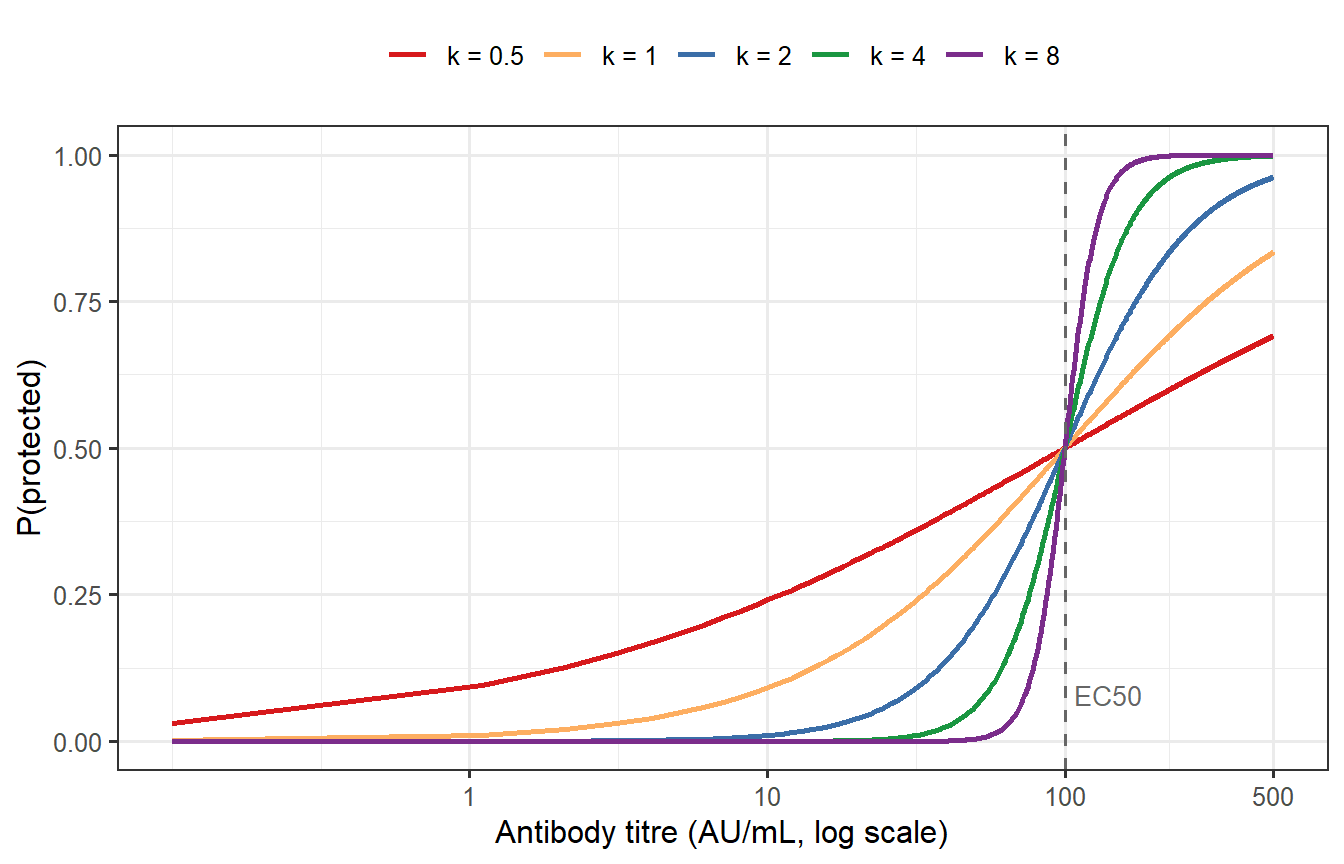
```{r hill-shapes, fig.cap="The Hill protection model for EC50 = 100 and varying Hill coefficients k. Low k (blue) gives a gentle, gradual protection curve — even individuals with low titres have some protection and even high titres give incomplete protection. High k (red) gives a near-binary threshold: most individuals with titre above EC50 are fully protected, most below are not. For COVID-19 vaccines, k ≈ 2–3 was estimated from meta-analysis."}
titre_grid <- seq(0.1, 500, length.out = 500)
EC50_ref   <- 100

k_vals <- c(0.5, 1, 2, 4, 8)
df_hill <- expand.grid(titre = titre_grid, k = k_vals) |>
  mutate(
    P_protect = titre^k / (titre^k + EC50_ref^k),
    k_label   = factor(paste0("k = ", k), levels = paste0("k = ", k_vals))
  )

pal_k <- c("k = 0.5" = "#D7191C", "k = 1" = "#FDAE61",
           "k = 2"   = "#3B6EA8", "k = 4" = "#1A9641", "k = 8" = "#7B2D8B")

ggplot(df_hill, aes(x = titre, y = P_protect, colour = k_label)) +
  geom_line(linewidth = 0.9) +
  geom_vline(xintercept = EC50_ref, linetype = "dashed", colour = "grey40") +
  annotate("text", x = EC50_ref + 8, y = 0.08, label = "EC50",
           colour = "grey40", size = 3.5, hjust = 0) +
  scale_x_log10(breaks = c(1, 10, 100, 500),
                labels = c("1", "10", "100", "500")) +
  scale_colour_manual(values = pal_k) +
  labs(x = "Antibody titre (AU/mL, log scale)",
       y = "P(protected)",
       colour = NULL) +
  theme(legend.position = "top")
```
The Hill coefficient $k$ has a direct practical interpretation: it determines whether protection is **graded** (low $k$) or **threshold-like** (high $k$). A graded CoP means that even low-titre individuals have meaningful partial protection; a threshold CoP means the vaccine either works or does not, with little in-between. For COVID-19, empirical estimates cluster around $k \approx 2$–3 [@khoury2021; @cromer2022], intermediate between these extremes but closer to threshold-like.
---
# Fitting a CoP model from trial data
## Simulated trial data
We generate a synthetic cohort of 500 vaccinated trial participants. Each participant has a peak antibody titre drawn from a log-normal distribution (approximating BNT162b2 immunogenicity data), and an infection outcome determined by the Hill model with known ground-truth parameters.
```{r simulate-data}
set.seed(2024)
n_trial <- 500

# Titre distribution (log-normal; median ≈ 150 AU/mL, ~4-fold inter-individual spread)
mu_log    <- log(150)
sigma_log <- 0.7
titre_obs <- rlnorm(n_trial, meanlog = mu_log, sdlog = sigma_log)

# True CoP parameters (ground truth; inspired by Khoury et al. 2021)
EC50_true <- 120
k_true    <- 2.2

hill_p <- function(T, EC50, k) T^k / (T^k + EC50^k)

p_protect_true <- hill_p(titre_obs, EC50_true, k_true)
infected       <- rbinom(n_trial, 1, prob = 1 - p_protect_true)  # 1 = infected

cat(sprintf(
  "Trial: %d participants, %d infected (%.1f%%), %d protected (%.1f%%)\n",
  n_trial, sum(infected), 100 * mean(infected),
  sum(infected == 0), 100 * mean(infected == 0)
))
```
## Maximum likelihood estimation
The Hill model is fitted by maximising the Bernoulli log-likelihood over $\text{EC}_{50}$ and $k$. Working on the log scale ensures parameters remain positive throughout optimisation.
```{r mle-fit}
neg_ll <- function(params) {
  EC50 <- exp(params[1])
  k    <- exp(params[2])
  p    <- hill_p(titre_obs, EC50, k)
  ll   <- sum(log(ifelse(infected == 0, p, 1 - p) + 1e-12))
  -ll
}

opt <- optim(c(log(100), log(2)), neg_ll, method = "BFGS", hessian = TRUE)

EC50_hat <- exp(opt$par[1])
k_hat    <- exp(opt$par[2])

cat(sprintf("True:      EC50 = %.1f,  k = %.2f\n", EC50_true, k_true))
cat(sprintf("Estimated: EC50 = %.1f, k = %.2f\n", EC50_hat, k_hat))
```
## Bootstrap confidence intervals
```{r bootstrap-ci, cache=TRUE}
set.seed(99)
n_boot <- 1000

boot_pars <- t(replicate(n_boot, {
  idx <- sample(n_trial, n_trial, replace = TRUE)
  neg_ll_b <- function(params) {
    EC50 <- exp(params[1]); k <- exp(params[2])
    p    <- hill_p(titre_obs[idx], EC50, k)
    -sum(log(ifelse(infected[idx] == 0, p, 1 - p) + 1e-12))
  }
  res <- tryCatch(
    optim(opt$par, neg_ll_b, method = "BFGS")$par,
    error = function(e) opt$par
  )
  exp(res)
}))

ci_EC50 <- quantile(boot_pars[, 1], c(0.025, 0.975))
ci_k    <- quantile(boot_pars[, 2], c(0.025, 0.975))

cat(sprintf("EC50: %.1f  (95%% CI: %.1f – %.1f)\n", EC50_hat, ci_EC50[1], ci_EC50[2]))
cat(sprintf("k: %.2f (95%% CI: %.2f – %.2f)\n", k_hat, ci_k[1], ci_k[2]))
```
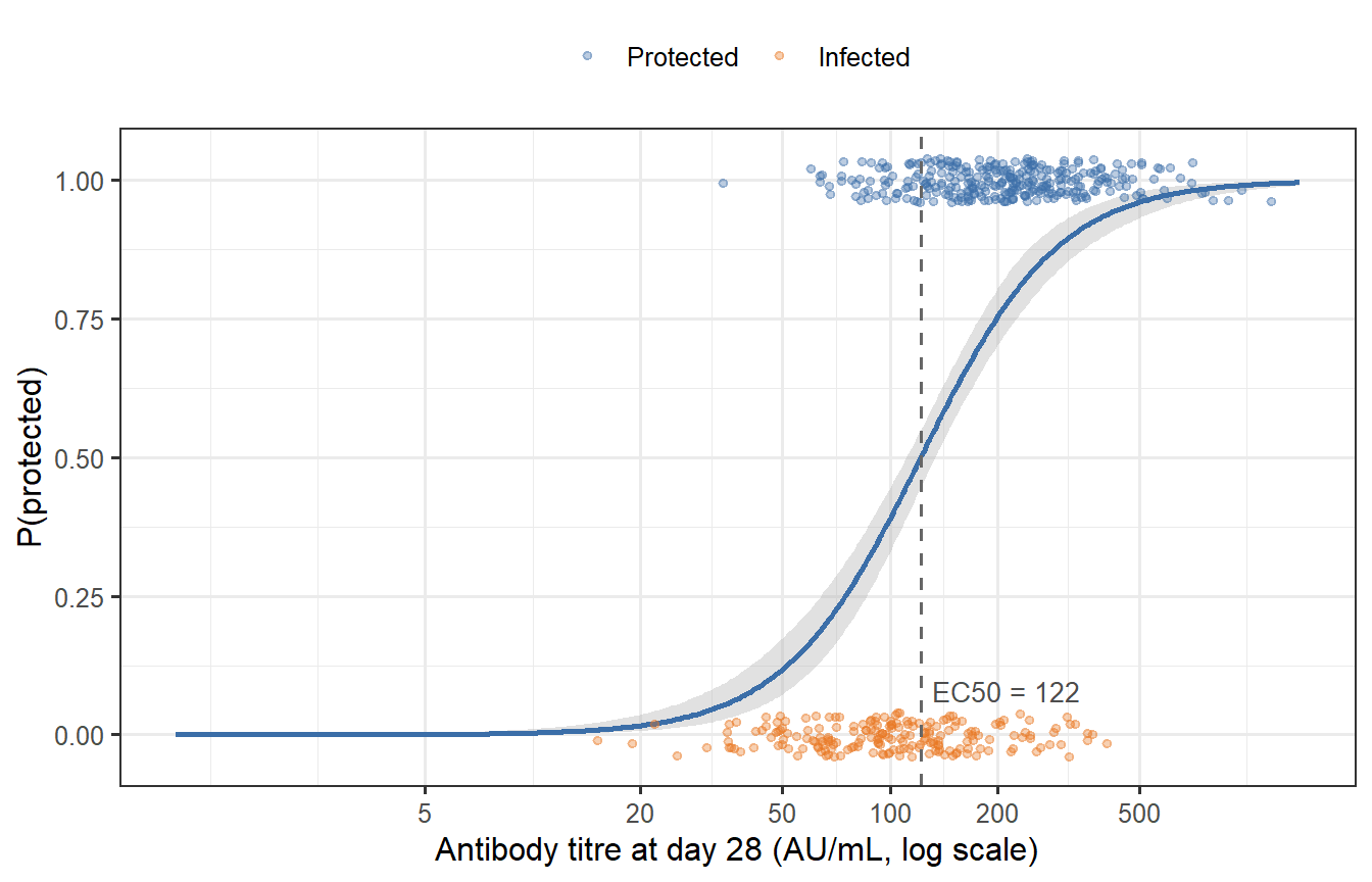
```{r cop-fit-plot, fig.cap="Fitted Hill model (solid curve) against simulated trial data. Points are jittered vertically; orange = infected, blue = protected. The grey band is the 95% bootstrap confidence interval around the fitted curve. The dashed line marks the estimated EC50."}
titre_seq <- exp(seq(log(1), log(max(titre_obs) * 1.2), length.out = 400))

# Bootstrap uncertainty band
band_mat <- apply(boot_pars, 1, function(p) hill_p(titre_seq, p[1], p[2]))
p_lo <- apply(band_mat, 1, quantile, 0.025)
p_hi <- apply(band_mat, 1, quantile, 0.975)

df_curve <- tibble(
  titre  = titre_seq,
  p_fit  = hill_p(titre_seq, EC50_hat, k_hat),
  p_lo   = p_lo,
  p_hi   = p_hi
)

df_pts <- tibble(
  titre    = titre_obs,
  outcome  = factor(ifelse(infected == 0, "Protected", "Infected"),
                    levels = c("Protected", "Infected")),
  y_jitter = ifelse(infected == 0, 1, 0) + runif(n_trial, -0.04, 0.04)
)

ggplot() +
  geom_ribbon(data = df_curve,
              aes(x = titre, ymin = p_lo, ymax = p_hi),
              fill = "grey70", alpha = 0.4) +
  geom_line(data = df_curve, aes(x = titre, y = p_fit),
            colour = "#3B6EA8", linewidth = 1.0) +
  geom_point(data = df_pts,
             aes(x = titre, y = y_jitter, colour = outcome),
             alpha = 0.35, size = 1.2) +
  geom_vline(xintercept = EC50_hat, linetype = "dashed", colour = "grey40") +
  annotate("text", x = EC50_hat * 1.08, y = 0.08,
           label = sprintf("EC50 = %.0f", EC50_hat),
           colour = "grey30", size = 3.5, hjust = 0) +
  scale_x_log10(breaks = c(5, 20, 50, 100, 200, 500),
                labels = c("5", "20", "50", "100", "200", "500")) +
  scale_colour_manual(values = c("Protected" = "#3B6EA8", "Infected" = "#E87722")) +
  labs(x = "Antibody titre at day 28 (AU/mL, log scale)",
       y = "P(protected)",
       colour = NULL) +
  theme(legend.position = "top")
```
The MLE recovers the ground-truth parameters well, and the bootstrap band is reassuringly narrow across the central range of titres — where most of the data lie. The band widens substantially at the extremes, reflecting the limited information content of data from individuals who are almost certainly protected (high titre) or almost certainly susceptible (very low titre).
---
# Time-varying protection
The CoP model so far treats titre as a static snapshot at day 28. But titre changes over time — as shown in Post 1 — and so does protection. Combining the within-host ODE with the CoP gives us a **continuous protection trajectory**: $P(\text{protected} \mid t) = P(\text{protected} \mid \text{Ab}(t))$.
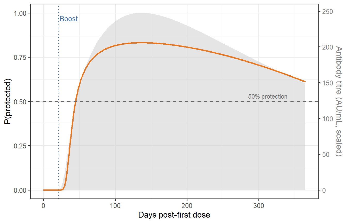
```{r time-protection, fig.cap="Time-varying protection for a representative vaccinated individual (prime-boost at days 0 and 21). The antibody trajectory from Post 1's ODE model (grey, right axis) is scaled to titre units and fed into the fitted Hill CoP. The orange curve shows P(protected) over 12 months. The dashed horizontal line marks the 50% protection level corresponding to EC50. Protection peaks at ~85% around day 35–40, then wanes slowly, remaining above 50% for most of the year thanks to the long-lived plasma cell pool."}
# Scale Ab trajectory to titre units:
# set peak prime-boost Ab = 200 AU/mL (approximately 90th percentile of our cohort)
peak_ab    <- max(out_pb$Ab)
ref_titre  <- quantile(titre_obs, 0.75)   # ~75th percentile titre
scale_fac  <- ref_titre / peak_ab

df_traj <- out_pb |>
  mutate(
    titre_scaled = Ab * scale_fac,
    P_protect    = hill_p(titre_scaled, EC50_hat, k_hat)
  )

# Dual-axis plot
y_ab_max <- max(df_traj$titre_scaled)
y_p_max  <- 1

p_traj <- ggplot(df_traj, aes(x = time)) +
  geom_area(aes(y = titre_scaled / y_ab_max),
            fill = "grey80", alpha = 0.5) +
  geom_line(aes(y = P_protect),
            colour = "#E87722", linewidth = 1.0) +
  geom_hline(yintercept = 0.5, linetype = "dashed", colour = "grey40") +
  geom_vline(xintercept = 21, linetype = "dotted", colour = "#3B6EA8",
             linewidth = 0.7) +
  annotate("text", x = 23, y = 0.97, label = "Boost", colour = "#3B6EA8",
           size = 3.5, hjust = 0) +
  annotate("text", x = 340, y = 0.53, label = "50% protection",
           colour = "grey40", size = 3, hjust = 1) +
  scale_y_continuous(
    name    = "P(protected)",
    limits  = c(0, 1),
    sec.axis = sec_axis(~ . * y_ab_max,
                        name = "Antibody titre (AU/mL, scaled)")
  ) +
  labs(x = "Days post-first dose") +
  theme(axis.title.y.right = element_text(colour = "grey50"),
        axis.text.y.right  = element_text(colour = "grey50"))

p_traj
```
This figure encodes a key insight for trial design: **the time window of adequate protection is not simply determined by when titres fall, but by the shape of the CoP curve and where the individual sits on it**. An individual whose titre starts high may remain above 50% protection for 10+ months; someone in the bottom quartile of the immunogenicity distribution may drop below that threshold within 3–4 months post-boost.
A digital twin makes this explicit and individual-specific — unlike population-average efficacy estimates that obscure the heterogeneity.
---
# From individual titres to population vaccine efficacy
## Building a mini virtual patient cohort
A single representative patient is illustrative but not sufficient for trial design. We need a *distribution* of patients — a virtual patient cohort. Post 3 will build this properly using Latin hypercube sampling across all ODE parameters. For now, we demonstrate the concept by varying the SLPC stimulation rate $k_S$, the dominant determinant of peak antibody titre.
```{r virtual-cohort, cache=TRUE}
set.seed(777)
n_vp <- 300

# Log-normal multiplier on kS: ~2-fold individual variation in peak titre
kS_mult <- rlnorm(n_vp, meanlog = 0, sdlog = 0.45)

# Simulate ODE for each virtual patient; extract peak titre
vp_peaks <- vapply(kS_mult, function(m) {
  p_i <- parms_wh
  p_i["kS"] <- parms_wh["kS"] * m
  out_i <- as.data.frame(ode(y = state0, times = times_wh,
                              func = withinhost_vax, parms = p_i,
                              events = list(data = dose2)))
  max(out_i$Ab) * scale_fac   # convert to titre units
}, numeric(1))

# Protection probability at peak titre for each virtual patient
vp_protect <- hill_p(vp_peaks, EC50_hat, k_hat)
```
## Population VE from individual heterogeneity
In a randomised trial comparing vaccinated to unvaccinated (placebo) participants, vaccine efficacy is:
$$
\text{VE} = 1 - \frac{P(\text{infection} \mid \text{vaccinated})}{P(\text{infection} \mid \text{unvaccinated})}
$$
Under 100% exposure (every participant encounters the pathogen), $P(\text{infection} \mid \text{vaccinated}) = 1 - \bar{P}$ where $\bar{P}$ is the mean individual protection probability, and $P(\text{infection} \mid \text{unvaccinated}) = 1$. Therefore:
$$
\text{VE} = \bar{P} = \frac{1}{n} \sum_i P(\text{protected} \mid T_i)
$$
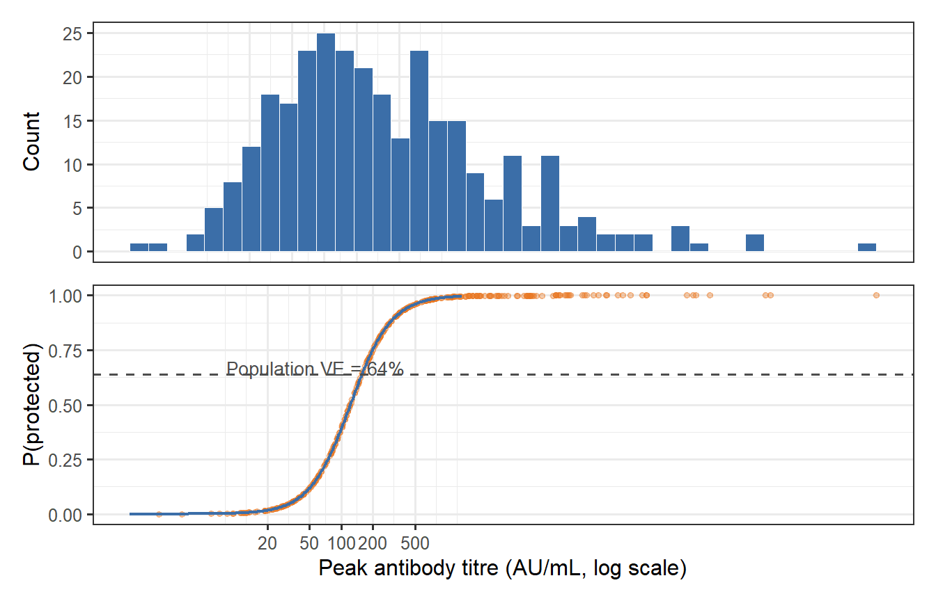
```{r ve-heterogeneity, fig.cap="Virtual patient cohort: distribution of peak antibody titres (top) and individual protection probabilities (bottom). The population VE (dashed line) is the mean of the individual protection probabilities — but its value is sensitive to the entire distribution, not just the mean titre. The long left tail of poorly protected individuals (low P_protect) pulls population VE below what you would calculate by plugging the mean titre into the Hill model."}
VE_pop      <- mean(vp_protect)
VE_mean_tit <- hill_p(mean(vp_peaks), EC50_hat, k_hat)   # naive: plug in mean titre

cat(sprintf("Population VE (mean of P_i):   %.1f%%\n", 100 * VE_pop))
cat(sprintf("Naive VE (Hill at mean titre): %.1f%%\n", 100 * VE_mean_tit))
df_vp <- tibble(titre = vp_peaks, P_protect = vp_protect)

p_hist <- ggplot(df_vp, aes(x = titre)) +
  geom_histogram(bins = 40, fill = "#3B6EA8", colour = "white", linewidth = 0.2) +
  scale_x_log10(breaks = c(20, 50, 100, 200, 500),
                labels = c("20", "50", "100", "200", "500")) +
  labs(x = NULL, y = "Count") +
  theme(axis.text.x = element_blank(), axis.ticks.x = element_blank())

p_prot <- ggplot(df_vp, aes(x = titre, y = P_protect)) +
  geom_point(alpha = 0.35, colour = "#E87722", size = 1.2) +
  geom_line(data = df_curve, aes(x = titre, y = p_fit),
            colour = "#3B6EA8", linewidth = 0.8) +
  geom_hline(yintercept = VE_pop, linetype = "dashed", colour = "grey30") +
  annotate("text", x = 400, y = VE_pop + 0.03,
           label = sprintf("Population VE = %.0f%%", 100 * VE_pop),
           colour = "grey30", size = 3.5, hjust = 1) +
  scale_x_log10(breaks = c(20, 50, 100, 200, 500),
                labels = c("20", "50", "100", "200", "500")) +
  labs(x = "Peak antibody titre (AU/mL, log scale)", y = "P(protected)")

p_hist / p_prot
```
The calculation surfaces a subtle but important result: **plugging the mean titre into the Hill model overestimates population VE**. The correct calculation integrates over the titre distribution, and the non-linearity of the Hill model means the left tail (low-titre, poorly protected individuals) drags the population average down disproportionately. This Jensen's inequality effect is one reason why "mean immunogenicity → mean efficacy" reasoning can be misleading in vaccine development.
The discrepancy is largest when:
1. The titre distribution is wide (high $\sigma_{\log}$), so the left tail is large.
2. The Hill coefficient $k$ is moderate (the CoP curve is non-linear but not binary).
3. The mean titre sits near $\text{EC}_{50}$, in the steepest part of the curve.
A digital twin that samples individual patients from their titre distribution — rather than working with population averages — gets this right automatically.
---
# Implications for trial design
The CoP model quantifies several things that matter directly for trial planning:
**1. Predicted vaccine efficacy before Phase 3.** If you have Phase 1/2 immunogenicity data (titre distributions) and a CoP estimated from earlier trials or challenge studies, you can predict Phase 3 VE before enrolling a single patient. This is the most commercially valuable use of the CoP model: it informs go/no-go decisions and dose selection.
**2. The correlate as a primary endpoint.** Regulatory guidance increasingly allows immunogenicity endpoints (titre above a CoP threshold) as primary endpoints for bridging studies and booster approvals. FDA used this framework to approve SARS-CoV-2 booster doses in children without new efficacy trials.
**3. Time-to-booster decisions.** The time-varying protection curve shows when the mean (or any percentile) patient drops below a given protection threshold. This is how booster timing policies are now being designed — not from expert opinion but from quantitative model predictions.
**4. Subgroup analysis.** The CoP curve applied to different subgroup titre distributions predicts differential efficacy in elderly, immunocompromised, or previously infected populations — a direct input to trial stratification and eligibility criteria.
---
# What comes next
We now have two of the three building blocks of a vaccine digital twin:
1. ✅ **Post 1**: A within-host ODE that generates $\text{Ab}(t)$ for any given parameter set.
2. ✅ **Post 2** (this post): A CoP model that maps $\text{Ab}(t) \to P(\text{protected at time } t)$.
The missing piece is **inter-individual variability**: the fact that different people have very different within-host parameters, and we need to represent this variation realistically. In Post 3, we build a proper **virtual patient cohort** by sampling parameter uncertainty with Latin hypercube methods, calibrating to observed immunogenicity distributions, and validating that the resulting virtual population reproduces trial immunogenicity data.
---
# References {.unnumbered}
::: {#refs}
:::
```{r session-info, echo=FALSE}
sessionInfo()
```