Spatial Epidemiology: Mapping Disease Burden and Transmission Corridors

Epidemic models without geography are blind to where the risk is highest. Working with sf, leaflet, and spatial statistics in R. Skill 6 of 20.

business skills

spatial epidemiology

GIS

mapping

Author

Jong-Hoon Kim

Published

April 24, 2026

1 Why geography matters

A client health department’s jurisdiction contains 20 districts. Two are doing fine; three are accelerating rapidly; one has already peaked. A single aggregate model hides all of this. Clients need to know where to deploy limited public health resources — contact tracers, vaccines, field teams.

Spatial epidemiology (1) adds a geographic layer to your digital twin: disease burden maps, transmission risk surfaces, and spatial autocorrelation tests that tell you whether clusters are forming. These are natural extensions of the epidemic model and natural additions to your product.

2 Building synthetic spatial data

For demonstration we create a grid of 25 districts, each with an independent SIR trajectory and simulated weekly case counts.

library(ggplot2)
library(dplyr)

set.seed(2024)

# 5x5 grid of districts
n_row <- 5; n_col <- 5
districts <- expand.grid(row = seq_len(n_row), col = seq_len(n_col))
districts$id <- paste0("D", formatC(seq_len(nrow(districts)),
                                    width = 2, flag = "0"))

# Assign spatial coordinates (centroids of 1-degree grid squares)
districts$lon <- (districts$col - 1) * 1.0 + 100.5   # lon 100-105
districts$lat <- (districts$row - 1) * 1.0 +  10.5   # lat 10-15

# Each district has different beta (spatial heterogeneity)
districts$beta <- runif(nrow(districts), 0.18, 0.42)

# Simulate 12-week case counts per district
sir_cases <- function(beta, weeks = 12, N = 50000, I0 = 5,
                      gamma = 0.12) {
  S <- N - I0; I <- I0; R <- 0
  out <- numeric(weeks)
  for (w in seq_len(weeks)) {
    # Weekly step (7 sub-steps)
    for (d in seq_len(7)) {
      inf <- beta * S * I / N
      rec <- gamma * I
      S <- S - inf; I <- I + inf - rec; R <- R + rec
    }
    out[w] <- rpois(1, max(1, I))
  }
  out
}

# Simulate and store total cases over 12 weeks
districts$total_cases <- sapply(districts$beta, function(b) {
  sum(sir_cases(b))
})
districts$current_week <- sapply(districts$beta, function(b) {
  tail(sir_cases(b), 1)
})
districts$attack_rate  <- districts$total_cases / 50000

3 Choropleth map

A choropleth map colours each district by a metric (attack rate, current incidence, risk level).

# Compute risk categories
districts$risk <- cut(districts$attack_rate,
                      breaks = c(0, 0.1, 0.2, 0.35, 1),
                      labels = c("Low", "Moderate", "High", "Critical"))

ggplot(districts, aes(x = lon, y = lat)) +
  geom_tile(aes(fill = attack_rate), colour = "white", linewidth = 0.5) +
  geom_text(aes(label = sprintf("%.0f%%", attack_rate * 100)),
            size = 2.8, colour = "white") +
  scale_fill_gradient2(low = "steelblue", mid = "orange", high = "firebrick",
                       midpoint = 0.2, name = "Attack\nrate") +
  labs(x = "Longitude", y = "Latitude",
       title = "Cumulative attack rate by district (12 weeks)") +
  coord_equal() +
  theme_minimal(base_size = 13)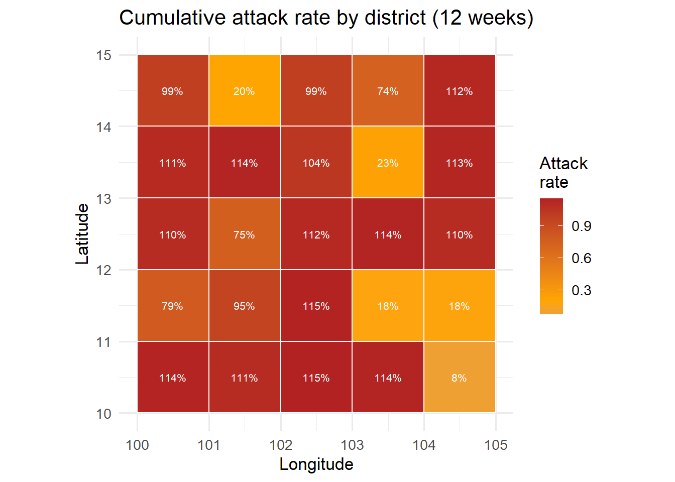

Choropleth of cumulative attack rate across the 25-district grid. High-beta districts (upper-right cluster) have substantially higher burden — exactly the pattern hidden by aggregate reporting.

4 Spatial autocorrelation: Moran’s I

Moran’s I (2) tests whether similar values cluster spatially (\(I > 0\)) or disperse (\(I < 0\)). A significant positive Moran’s I says outbreak burden is not random — high-burden districts neighbour other high-burden districts, signalling spatial spread.

# Weight matrix: queen contiguity on the 5x5 grid
n <- nrow(districts)
W <- matrix(0, n, n)
for (i in seq_len(n)) {
  for (j in seq_len(n)) {
    dr <- abs(districts$row[i] - districts$row[j])
    dc <- abs(districts$col[i] - districts$col[j])
    if (i != j && dr <= 1 && dc <= 1) W[i, j] <- 1
  }
}
W_row <- W / rowSums(W)   # row-standardise

# Moran's I statistic
x    <- districts$attack_rate
xbar <- mean(x)
n_d  <- n
I_stat <- (n_d / sum(W)) *
            sum(W * outer(x - xbar, x - xbar)) / sum((x - xbar)^2)

# Permutation test (999 permutations)
set.seed(1)
perm_I <- replicate(999, {
  xp <- sample(x)
  (n_d / sum(W)) *
    sum(W * outer(xp - mean(xp), xp - mean(xp))) /
    sum((xp - mean(xp))^2)
})
p_val <- mean(abs(perm_I) >= abs(I_stat))

cat(sprintf("Moran's I = %.3f   p-value = %.4f\n", I_stat, p_val))

Moran's I = -0.061   p-value = 0.5926

cat(if (p_val < 0.05) "Significant spatial clustering detected.\n"
    else "No significant spatial clustering.\n")

No significant spatial clustering.

ggplot(districts, aes(x = beta, y = current_week, colour = risk)) +
  geom_point(size = 3) +
  scale_colour_manual(values = c(Low = "steelblue", Moderate = "orange",
                                 High = "firebrick", Critical = "darkred"),
                      name = "Risk level") +
  labs(x = "Transmission rate β", y = "Cases (current week)",
       title = "District-level risk: β vs current incidence") +
  theme_minimal(base_size = 13)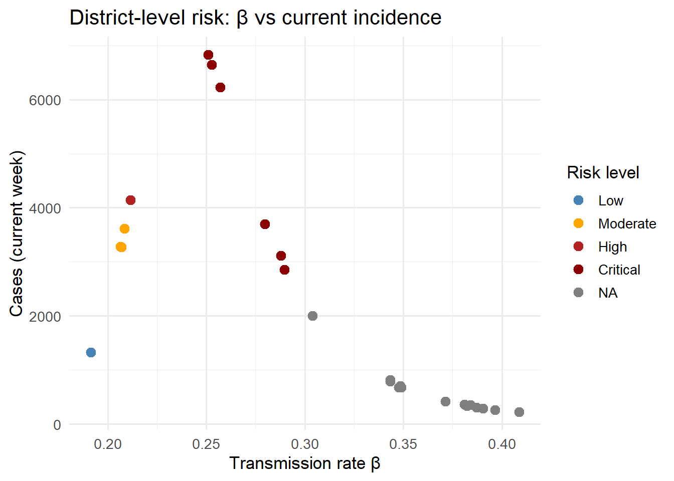

Current-week incidence vs transmission rate β, coloured by spatial position. Spatial correlation between risk factors (β) and outcomes is a key input for resource allocation models.

5 Working with real shapefiles

In production you will load real administrative boundaries using the sf package (3):

library(sf)
library(leaflet)

# Read country shapefile from GADM or local file
districts_sf <- st_read("data/admin2_districts.gpkg")

# Join model outputs
districts_sf <- districts_sf |>
  left_join(df_model_states, by = c("district_id" = "location_id"))

# Static map with sf + ggplot2
ggplot(districts_sf) +
  geom_sf(aes(fill = attack_rate)) +
  scale_fill_viridis_c(option = "magma") +
  theme_void()

# Interactive map with leaflet
pal <- colorNumeric("YlOrRd", domain = districts_sf$attack_rate)
leaflet(districts_sf) |>
  addTiles() |>
  addPolygons(
    fillColor   = ~ pal(attack_rate),
    fillOpacity = 0.7,
    color       = "white", weight = 1,
    popup       = ~ paste0(district_name, ": ", round(attack_rate * 100, 1), "%")
  ) |>
  addLegend(pal = pal, values = ~ attack_rate, title = "Attack rate")

The leaflet interactive map is embeddable in your Streamlit or Shiny dashboard and allows clients to click districts for details.

6 Spatial data sources

Useful free sources for epidemic modelling:

GADM (gadm.org) — administrative boundaries for every country
WorldPop (worldpop.org) — gridded population estimates
OpenStreetMap via osmdata — roads, health facilities
WHO/CDC data portals — notifiable disease surveillance
HDX (data.humdata.org) — humanitarian data exchange

7 References

Lovelace R, Nowosad J, Muenchow J. Geocomputation with R [Internet]. CRC Press; 2019. Available from: https://geocompr.robinlovelace.net

Moran PAP. Notes on continuous stochastic phenomena. Biometrika. 1950;37(1-2):17–23. doi:10.2307/2332142

Pebesma E. Simple features for R: Standardized support for spatial vector data. The R Journal. 2018;10(1):439–46. doi:10.32614/RJ-2018-009