A Lightweight Data Lake for Epidemic Surveillance Ingestion
Hospital data, wastewater, and syndromic surveillance land in different formats. Parquet + DuckDB unifies them into one queryable store. Skill 12 of 20.
business skills
data engineering
Parquet
DuckDB
Arrow
R
Author
Jong-Hoon Kim
Published
April 24, 2026
1 The heterogeneous data problem
A real-time epidemic digital twin ingests from multiple sources simultaneously:
Hospital: daily admissions CSV emailed at 8 AM
Wastewater: JSON from lab API, updated 3×/week
Syndromic surveillance: nightly SQL dump from the health information system
Routing all of these directly into TimescaleDB requires a schema for each, an ingestion script for each, and a way to handle delays, duplicates, and format changes. The classic data engineering pattern is to land raw data in a data lake first — a cheap, schema-flexible storage layer — and then push cleaned, normalised records to the model database.
2 The Parquet + DuckDB stack
Parquet(1) is a column-oriented file format with efficient compression. A 100MB CSV typically compresses to 10–20MB Parquet with dramatically faster analytical queries.
DuckDB(2) is an in-process analytical database that queries Parquet files directly — no server required. Together they implement a lightweight data lake that runs on a single EC2 instance.
Raw files (S3 or local)
  hospital/2024-04-01.csv
  wastewater/2024-04-01.json
  syndromic/2024-04-01.parquet
         │
         ▼  (ingestion scripts)
Landing zone  → Parquet partitioned by source + date
         │
         ▼  (DuckDB transform query)
Cleaned layer → Normalised Parquet schema
         │
         ▼
TimescaleDB   → observations table
3 Building the ingestion pipeline in R
library(dplyr)# Simulate raw data from three heterogeneous sourcesset.seed(2024)n_days <-14dates <-seq(as.Date("2024-04-01"), by ="day", length.out = n_days)# Source 1: hospital admissions (CSV-like: district, date, admissions)df_hospital <-data.frame(District =rep(c("North", "South"), each = n_days),ReportDate =rep(dates, 2),Admissions =rpois(n_days *2, 30),DataVersion ="v2.1")# Source 2: wastewater (JSON-like: different naming, units)df_ww <-data.frame(district_code =rep(c("N", "S"), each = n_days),sample_date =rep(dates, 2),gc_per_ml =round(runif(n_days *2, 100, 5000)),lab_id ="WW_LAB_001")# Source 3: syndromic surveillance (SQL dump: ICD-coded ED visits)df_syndromic <-data.frame(location =rep(c("North", "South"), each = n_days),visit_dt =rep(dates, 2),icd_flu =rpois(n_days *2, 15),icd_resp =rpois(n_days *2, 45))cat("Hospital rows:", nrow(df_hospital)," | WW rows:", nrow(df_ww)," | Syndromic rows:", nrow(df_syndromic), "\n")
        date location_id   source     metric value
1 2024-04-01       north hospital admissions    35
2 2024-04-02       north hospital admissions    32
3 2024-04-03       north hospital admissions    29
4 2024-04-04       north hospital admissions    28
# In production: write to Parquet and query with DuckDBlibrary(arrow)library(duckdb)# Write partitioned Parquet (partitioned by source + date)write_dataset(df_lake, path ="data_lake/cleaned",format ="parquet",partitioning =c("source", "date"))# Query with DuckDB — no need to load into memorycon <-dbConnect(duckdb::duckdb())dbExecute(con, " CREATE VIEW lake AS SELECT * FROM parquet_scan('data_lake/cleaned/**/*.parquet', hive_partitioning = TRUE)")# Aggregate across sourcesresult <-dbGetQuery(con, " SELECT date, location_id, source, SUM(value) AS total FROM lake WHERE metric IN ('admissions', 'flu_ed_visits') GROUP BY date, location_id, source ORDER BY date, location_id")dbDisconnect(con)
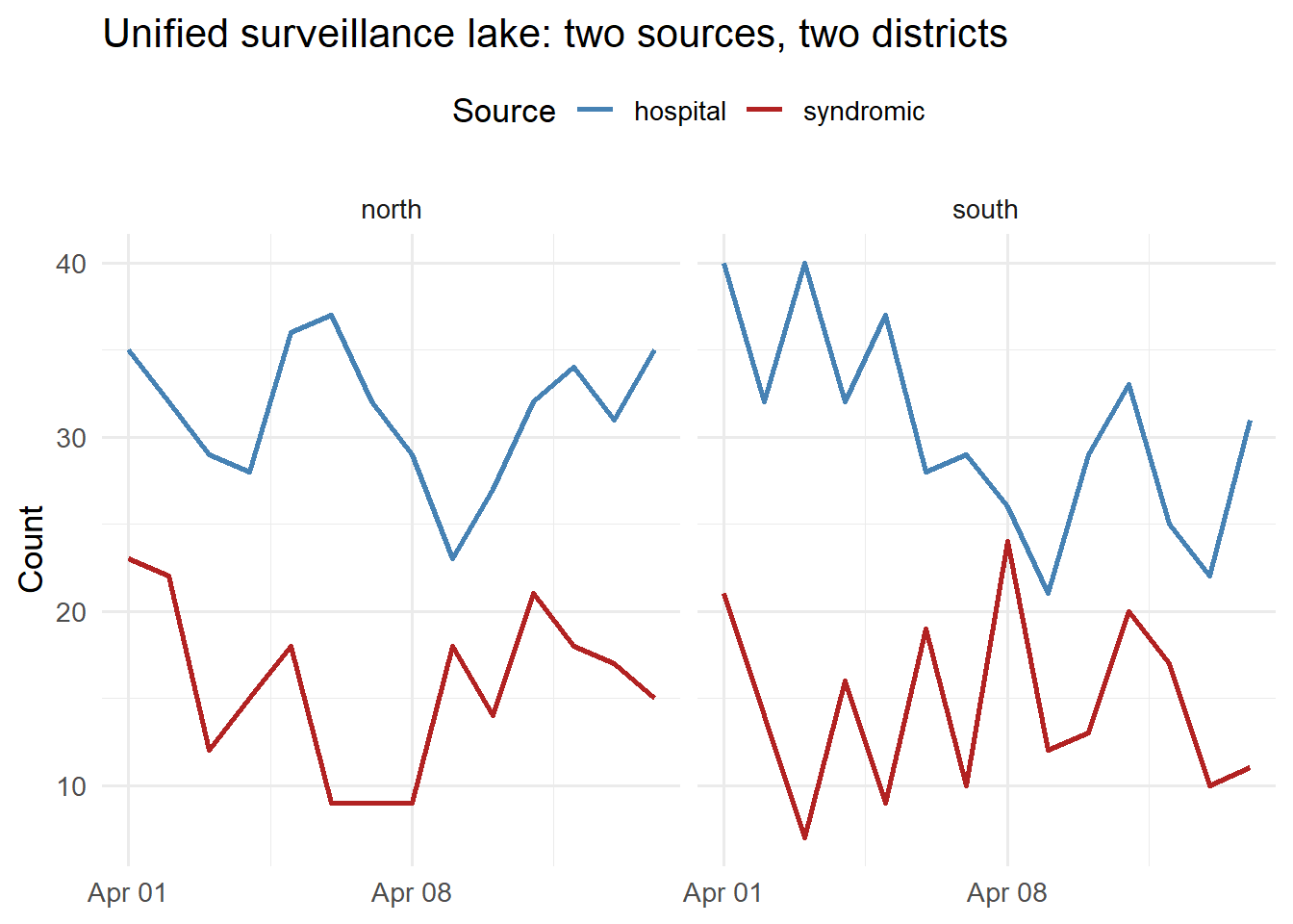
library(ggplot2)ggplot(df_lake |>filter(metric %in%c("admissions","flu_ed_visits")),aes(x = date, y = value, colour = source)) +geom_line(linewidth =1) +facet_wrap(~ location_id, ncol =2) +scale_colour_manual(values =c(hospital ="steelblue",syndromic ="firebrick"),name ="Source") +labs(x =NULL, y ="Count", title ="Unified surveillance lake: two sources, two districts") +theme_minimal(base_size =13) +theme(legend.position ="top")
Unified surveillance lake: three heterogeneous data sources normalised to a common schema and visualised together. This is the view your EnKF ingestion script queries each morning.
DuckDB’s partition pruning means a query filtered to source='hospital' AND date='2024-04-01' reads only a few kilobytes, even if the full lake is hundreds of gigabytes.
5 From lake to model
The EnKF runner queries the lake each morning:
# Pull yesterday's unified case counts for all districtsobs_today <- df_lake |>filter( date ==Sys.Date() -1, metric =="admissions", source =="hospital" ) |>arrange(location_id)# Feed into EnKFrun_enkf(obs_today$value, obs_today$location_id)
The lake is the contract between the messy world of surveillance data and the clean model pipeline that depends on it.